radar datatree: Cloud-native, time-aware weather radar datasets#
You want to look at how a Chicago-area storm evolved on a given date. The traditional path: download multiple gigabytes of NEXRAD Level II files, decode them, georeference each sweep, and stitch them together. This notebook does the same end-to-end, streaming straight from the cloud — connect, load, slice, georeference, plot.
Why a DataTree?#
Weather radar volumes are organized hierarchically: a Volume Coverage Pattern (VCP) cycles through several 360° sweeps at increasing elevation angles, repeating every 4–10 minutes. Different VCPs have different shapes, which is exactly what xarray.DataTree is built for.
Hierarchical — every VCP × sweep combination is a node you navigate (
dt["VCP-12/sweep_0"]), not a separate file you parse.Time-indexed — all scans share a
vcp_timedimension, so.sel(vcp_time=...)replaces the file-iteration loop.Lazy — opening the full archive fetches metadata only (~MB). Variables stream from object storage on demand.
For architecture and scaling benchmarks, see Ladino-Rincón et al. (2026, in preparation). Unfamiliar acronyms (VCP, polarimetric, ZDR, RHOHV, …) are all defined in the glossary.
radar datatree in practice#
Let’s see how the radar datatree looks in practice.
import sys
from pathlib import Path

# Make notebooks/demo_functions.py importable when sphinx-build runs the
# rendered docs page from docs/ (which is a symlink to ../notebooks/).
# Harmless on Colab — the bootstrap above fetches demo_functions.py into
# the kernel CWD, and a path that doesn't exist is silently ignored.
sys.path.insert(0, str(Path("../notebooks").resolve()))

from demo_functions import connect_to_nexrad_arco

# One-line connect to the public KLOT archive on AWS Open Data — anonymous
# S3 reads, no credentials needed. See the helper's docstring for the
# s3_storage / Repository.open / readonly_session boilerplate it wraps.
session = connect_to_nexrad_arco("KLOT")
print("Connected to s3://nexrad-arco/KLOT on branch 'main'")
Connected to s3://nexrad-arco/KLOT on branch 'main'
We can use xarray.open_datatree to explore the radar archive — with engine="rustytree", a Rust-backed xarray DataTree backend recommended for radar-datatree archives. It’s a drop-in replacement for the standard engine="zarr", ~10× faster on icechunk repos served from object storage (see rustytree-xarray on PyPI).
import xarray as xr
import xradar  # noqa: F401  — registers the .xradar accessor

dt = xr.open_datatree(session.store, engine="rustytree", chunks=None)
dt
<xarray.DataTree>
Group: /
├── Group: /VCP-112
│ │ Dimensions: (vcp_time: 108)
│ │ Coordinates:
│ │ * vcp_time (vcp_time) datetime64[ns] 864B 2020-11-05T13:16:18.795000 ...
│ │ altitude int64 8B ...
│ │ latitude float64 8B ...
│ │ longitude float64 8B ...
│ │ Data variables:
│ │ volume_number (vcp_time) float64 864B ...
│ │ Attributes:
│ │ Conventions: Cf/Radial instrument_parameters radar_parameters
│ │ attribution: NOAA NEXRAD Level 2 data processed by Atmoscale from NOAA O...
│ │ dataset_id: nexrad-arco-klot
│ │ institution: NOAA National Weather Service
│ │ source: WSR-88D S-band weather radar
│ │ time_domain: 2026-05-08 to Present
│ │ title: NEXRAD ARCO - KLOT
│ │ version: 2.1
│ ├── Group: /VCP-112/sweep_0
│ │ Dimensions: (vcp_time: 108, azimuth: 720, range: 1832)
│ │ Coordinates:
│ │ * azimuth (azimuth) float64 6kB 0.25 0.75 1.25 ... 359.2 359.8
│ │ elevation (azimuth) float64 6kB ...
│ │ time (vcp_time, azimuth) datetime64[ns] 622kB ...
│ │ * range (range) float32 7kB 2.125e+03 2.375e+03 ... 4.599e+05
│ │ Data variables:
│ │ CCORH (vcp_time, azimuth, range) float32 570MB ...
│ │ DBZH (vcp_time, azimuth, range) float32 570MB ...
│ │ PHIDP (vcp_time, azimuth, range) float32 570MB ...
│ │ RHOHV (vcp_time, azimuth, range) float32 570MB ...
│ │ ZDR (vcp_time, azimuth, range) float32 570MB ...
│ │ ray_elevation_angle (vcp_time, azimuth) float64 622kB ...
│ │ sweep_fixed_angle (vcp_time) float32 432B ...
│ │ sweep_number (vcp_time) float32 432B ...
│ ├── Group: /VCP-112/sweep_1
│ │ Dimensions: (vcp_time: 108, azimuth: 720, range: 1192)
│ │ Coordinates:
│ │ * azimuth (azimuth) float64 6kB 0.25 0.75 1.25 ... 359.2 359.8
│ │ elevation (azimuth) float64 6kB ...
│ │ time (vcp_time, azimuth) datetime64[ns] 622kB ...
│ │ * range (range) float32 5kB 2.125e+03 2.375e+03 ... 2.999e+05
│ │ Data variables:
│ │ DBZH (vcp_time, azimuth, range) float32 371MB ...
│ │ VRADH (vcp_time, azimuth, range) float32 371MB ...
│ │ WRADH (vcp_time, azimuth, range) float32 371MB ...
│ │ ray_elevation_angle (vcp_time, azimuth) float64 622kB ...
│ │ sweep_fixed_angle (vcp_time) float32 432B ...
│ │ sweep_number (vcp_time) float32 432B ...
│ ├── Group: /VCP-112/sweep_10
│ │ Dimensions: (vcp_time: 108, azimuth: 360, range: 1336)
│ │ Coordinates:
│ │ * azimuth (azimuth) float64 3kB 0.5 1.5 2.5 ... 357.5 358.5 359.5
│ │ elevation (azimuth) float64 3kB ...
│ │ time (vcp_time, azimuth) datetime64[ns] 311kB ...
│ │ * range (range) float32 5kB 2.125e+03 2.375e+03 ... 3.359e+05
│ │ Data variables:
│ │ CCORH (vcp_time, azimuth, range) float32 208MB ...
│ │ DBZH (vcp_time, azimuth, range) float32 208MB ...
│ │ PHIDP (vcp_time, azimuth, range) float32 208MB ...
│ │ RHOHV (vcp_time, azimuth, range) float32 208MB ...
│ │ VRADH (vcp_time, azimuth, range) float32 208MB ...
│ │ WRADH (vcp_time, azimuth, range) float32 208MB ...
│ │ ZDR (vcp_time, azimuth, range) float32 208MB ...
│ │ ray_elevation_angle (vcp_time, azimuth) float64 311kB ...
│ │ sweep_fixed_angle (vcp_time) float32 432B ...
│ │ sweep_number (vcp_time) float32 432B ...
│ ├── Group: /VCP-112/sweep_11
│ │ Dimensions: (vcp_time: 108, azimuth: 360, range: 1192)
│ │ Coordinates:
│ │ * azimuth (azimuth) float64 3kB 0.5 1.5 2.5 ... 357.5 358.5 359.5
│ │ elevation (azimuth) float64 3kB ...
│ │ time (vcp_time, azimuth) datetime64[ns] 311kB ...
│ │ * range (range) float32 5kB 2.125e+03 2.375e+03 ... 2.999e+05
│ │ Data variables:
│ │ CCORH (vcp_time, azimuth, range) float32 185MB ...
│ │ DBZH (vcp_time, azimuth, range) float32 185MB ...
│ │ PHIDP (vcp_time, azimuth, range) float32 185MB ...
│ │ RHOHV (vcp_time, azimuth, range) float32 185MB ...
│ │ VRADH (vcp_time, azimuth, range) float32 185MB ...
│ │ WRADH (vcp_time, azimuth, range) float32 185MB ...
│ │ ZDR (vcp_time, azimuth, range) float32 185MB ...
│ │ ray_elevation_angle (vcp_time, azimuth) float64 311kB ...
│ │ sweep_fixed_angle (vcp_time) float32 432B ...
│ │ sweep_number (vcp_time) float32 432B ...
│ ├── Group: /VCP-112/sweep_12
│ │ Dimensions: (vcp_time: 108, azimuth: 360, range: 1712)
│ │ Coordinates:
│ │ * azimuth (azimuth) float64 3kB 0.5 1.5 2.5 ... 357.5 358.5 359.5
│ │ elevation (azimuth) float64 3kB ...
│ │ time (vcp_time, azimuth) datetime64[ns] 311kB ...
│ │ * range (range) float32 7kB 2.125e+03 2.375e+03 ... 4.299e+05
│ │ Data variables:
│ │ CCORH (vcp_time, azimuth, range) float32 266MB ...
│ │ DBZH (vcp_time, azimuth, range) float32 266MB ...
│ │ PHIDP (vcp_time, azimuth, range) float32 266MB ...
│ │ RHOHV (vcp_time, azimuth, range) float32 266MB ...
│ │ VRADH (vcp_time, azimuth, range) float32 266MB ...
│ │ WRADH (vcp_time, azimuth, range) float32 266MB ...
│ │ ZDR (vcp_time, azimuth, range) float32 266MB ...
│ │ ray_elevation_angle (vcp_time, azimuth) float64 311kB ...
│ │ sweep_fixed_angle (vcp_time) float32 432B ...
│ │ sweep_number (vcp_time) float32 432B ...
│ ├── Group: /VCP-112/sweep_13
│ │ Dimensions: (vcp_time: 108, azimuth: 360, range: 824)
│ │ Coordinates:
│ │ * azimuth (azimuth) float64 3kB 0.5 1.5 2.5 ... 357.5 358.5 359.5
│ │ elevation (azimuth) float64 3kB ...
│ │ time (vcp_time, azimuth) datetime64[ns] 311kB ...
│ │ * range (range) float32 3kB 2.125e+03 2.375e+03 ... 2.079e+05
│ │ Data variables:
│ │ CCORH (vcp_time, azimuth, range) float32 128MB ...
│ │ DBZH (vcp_time, azimuth, range) float32 128MB ...
│ │ PHIDP (vcp_time, azimuth, range) float32 128MB ...
│ │ RHOHV (vcp_time, azimuth, range) float32 128MB ...
│ │ VRADH (vcp_time, azimuth, range) float32 128MB ...
│ │ WRADH (vcp_time, azimuth, range) float32 128MB ...
│ │ ZDR (vcp_time, azimuth, range) float32 128MB ...
│ │ ray_elevation_angle (vcp_time, azimuth) float64 311kB ...
│ │ sweep_fixed_angle (vcp_time) float32 432B ...
│ │ sweep_number (vcp_time) float32 432B ...
│ ...
│ ├── Group: /VCP-112/sweep_4
│ │ Dimensions: (vcp_time: 108, azimuth: 720, range: 1192)
│ │ Coordinates:
│ │ * azimuth (azimuth) float64 6kB 0.25 0.75 1.25 ... 359.2 359.8
│ │ elevation (azimuth) float64 6kB ...
│ │ time (vcp_time, azimuth) datetime64[ns] 622kB ...
│ │ * range (range) float32 5kB 2.125e+03 2.375e+03 ... 2.999e+05
│ │ Data variables:
│ │ DBZH (vcp_time, azimuth, range) float32 371MB ...
│ │ VRADH (vcp_time, azimuth, range) float32 371MB ...
│ │ WRADH (vcp_time, azimuth, range) float32 371MB ...
│ │ ray_elevation_angle (vcp_time, azimuth) float64 622kB ...
│ │ sweep_fixed_angle (vcp_time) float32 432B ...
│ │ sweep_number (vcp_time) float32 432B ...
│ ├── Group: /VCP-112/sweep_5
│ │ Dimensions: (vcp_time: 108, azimuth: 720, range: 1192)
│ │ Coordinates:
│ │ * azimuth (azimuth) float64 6kB 0.25 0.75 1.25 ... 359.2 359.8
│ │ elevation (azimuth) float64 6kB ...
│ │ time (vcp_time, azimuth) datetime64[ns] 622kB ...
│ │ * range (range) float32 5kB 2.125e+03 2.375e+03 ... 2.999e+05
│ │ Data variables:
│ │ DBZH (vcp_time, azimuth, range) float32 371MB ...
│ │ VRADH (vcp_time, azimuth, range) float32 371MB ...
│ │ WRADH (vcp_time, azimuth, range) float32 371MB ...
│ │ ray_elevation_angle (vcp_time, azimuth) float64 622kB ...
│ │ sweep_fixed_angle (vcp_time) float32 432B ...
│ │ sweep_number (vcp_time) float32 432B ...
│ ├── Group: /VCP-112/sweep_6
│ │ Dimensions: (vcp_time: 108, azimuth: 720, range: 1712)
│ │ Coordinates:
│ │ * azimuth (azimuth) float64 6kB 0.25 0.75 1.25 ... 359.2 359.8
│ │ elevation (azimuth) float64 6kB ...
│ │ time (vcp_time, azimuth) datetime64[ns] 622kB ...
│ │ * range (range) float32 7kB 2.125e+03 2.375e+03 ... 4.299e+05
│ │ Data variables:
│ │ CCORH (vcp_time, azimuth, range) float32 533MB ...
│ │ DBZH (vcp_time, azimuth, range) float32 533MB ...
│ │ PHIDP (vcp_time, azimuth, range) float32 533MB ...
│ │ RHOHV (vcp_time, azimuth, range) float32 533MB ...
│ │ ZDR (vcp_time, azimuth, range) float32 533MB ...
│ │ ray_elevation_angle (vcp_time, azimuth) float64 622kB ...
│ │ sweep_fixed_angle (vcp_time) float32 432B ...
│ │ sweep_number (vcp_time) float32 432B ...
│ ├── Group: /VCP-112/sweep_7
│ │ Dimensions: (vcp_time: 108, azimuth: 720, range: 1192)
│ │ Coordinates:
│ │ * azimuth (azimuth) float64 6kB 0.25 0.75 1.25 ... 359.2 359.8
│ │ elevation (azimuth) float64 6kB ...
│ │ time (vcp_time, azimuth) datetime64[ns] 622kB ...
│ │ * range (range) float32 5kB 2.125e+03 2.375e+03 ... 2.999e+05
│ │ Data variables:
│ │ DBZH (vcp_time, azimuth, range) float32 371MB ...
│ │ VRADH (vcp_time, azimuth, range) float32 371MB ...
│ │ WRADH (vcp_time, azimuth, range) float32 371MB ...
│ │ ray_elevation_angle (vcp_time, azimuth) float64 622kB ...
│ │ sweep_fixed_angle (vcp_time) float32 432B ...
│ │ sweep_number (vcp_time) float32 432B ...
│ ├── Group: /VCP-112/sweep_8
│ │ Dimensions: (vcp_time: 108, azimuth: 720, range: 1192)
│ │ Coordinates:
│ │ * azimuth (azimuth) float64 6kB 0.25 0.75 1.25 ... 359.2 359.8
│ │ elevation (azimuth) float64 6kB ...
│ │ time (vcp_time, azimuth) datetime64[ns] 622kB ...
│ │ * range (range) float32 5kB 2.125e+03 2.375e+03 ... 2.999e+05
│ │ Data variables:
│ │ DBZH (vcp_time, azimuth, range) float32 371MB ...
│ │ VRADH (vcp_time, azimuth, range) float32 371MB ...
│ │ WRADH (vcp_time, azimuth, range) float32 371MB ...
│ │ ray_elevation_angle (vcp_time, azimuth) float64 622kB ...
│ │ sweep_fixed_angle (vcp_time) float32 432B ...
│ │ sweep_number (vcp_time) float32 432B ...
│ └── Group: /VCP-112/sweep_9
│ Dimensions: (vcp_time: 108, azimuth: 360, range: 1712)
│ Coordinates:
│ * azimuth (azimuth) float64 3kB 0.5 1.5 2.5 ... 357.5 358.5 359.5
│ elevation (azimuth) float64 3kB ...
│ time (vcp_time, azimuth) datetime64[ns] 311kB ...
│ * range (range) float32 7kB 2.125e+03 2.375e+03 ... 4.299e+05
│ Data variables:
│ CCORH (vcp_time, azimuth, range) float32 266MB ...
│ DBZH (vcp_time, azimuth, range) float32 266MB ...
│ PHIDP (vcp_time, azimuth, range) float32 266MB ...
│ RHOHV (vcp_time, azimuth, range) float32 266MB ...
│ VRADH (vcp_time, azimuth, range) float32 266MB ...
│ WRADH (vcp_time, azimuth, range) float32 266MB ...
│ ZDR (vcp_time, azimuth, range) float32 266MB ...
│ ray_elevation_angle (vcp_time, azimuth) float64 311kB ...
│ sweep_fixed_angle (vcp_time) float32 432B ...
│ sweep_number (vcp_time) float32 432B ...
├── Group: /VCP-12
│ │ Dimensions: (vcp_time: 2573)
│ │ Coordinates:
│ │ * vcp_time (vcp_time) datetime64[ns] 21kB 2020-02-10T08:33:43.155000 ...
│ │ altitude int64 8B ...
│ │ latitude float64 8B ...
│ │ longitude float64 8B ...
│ │ Data variables:
│ │ volume_number (vcp_time) float64 21kB ...
│ │ Attributes:
│ │ Conventions: Cf/Radial instrument_parameters radar_parameters
│ │ attribution: NOAA NEXRAD Level 2 data processed by Atmoscale from NOAA O...
│ │ dataset_id: nexrad-arco-klot
│ │ institution: NOAA National Weather Service
│ │ source: WSR-88D S-band weather radar
│ │ time_domain: 2026-05-08 to Present
│ │ title: NEXRAD ARCO - KLOT
│ │ version: 2.1
│ ├── Group: /VCP-12/sweep_0
│ │ Dimensions: (vcp_time: 2573, azimuth: 720, range: 1832)
│ │ Coordinates:
│ │ * azimuth (azimuth) float64 6kB 0.25 0.75 1.25 ... 359.2 359.8
│ │ elevation (azimuth) float64 6kB ...
│ │ time (vcp_time, azimuth) datetime64[ns] 15MB ...
│ │ * range (range) float32 7kB 2.125e+03 2.375e+03 ... 4.599e+05
│ │ Data variables:
│ │ CCORH (vcp_time, azimuth, range) float32 14GB ...
│ │ DBZH (vcp_time, azimuth, range) float32 14GB ...
│ │ PHIDP (vcp_time, azimuth, range) float32 14GB ...
│ │ RHOHV (vcp_time, azimuth, range) float32 14GB ...
│ │ ZDR (vcp_time, azimuth, range) float32 14GB ...
│ │ ray_elevation_angle (vcp_time, azimuth) float64 15MB ...
│ │ sweep_fixed_angle (vcp_time) float32 10kB ...
│ │ sweep_number (vcp_time) float32 10kB ...
│ ├── Group: /VCP-12/sweep_1
│ │ Dimensions: (vcp_time: 2573, azimuth: 720, range: 1192)
│ │ Coordinates:
│ │ * azimuth (azimuth) float64 6kB 0.25 0.75 1.25 ... 359.2 359.8
│ │ elevation (azimuth) float64 6kB ...
│ │ time (vcp_time, azimuth) datetime64[ns] 15MB ...
│ │ * range (range) float32 5kB 2.125e+03 2.375e+03 ... 2.999e+05
│ │ Data variables:
│ │ DBZH (vcp_time, azimuth, range) float32 9GB ...
│ │ VRADH (vcp_time, azimuth, range) float32 9GB ...
│ │ WRADH (vcp_time, azimuth, range) float32 9GB ...
│ │ ray_elevation_angle (vcp_time, azimuth) float64 15MB ...
│ │ sweep_fixed_angle (vcp_time) float32 10kB ...
│ │ sweep_number (vcp_time) float32 10kB ...
│ ├── Group: /VCP-12/sweep_10
│ │ Dimensions: (vcp_time: 2573, azimuth: 360, range: 1336)
│ │ Coordinates:
│ │ * azimuth (azimuth) float64 3kB 0.5 1.5 2.5 ... 357.5 358.5 359.5
│ │ elevation (azimuth) float64 3kB ...
│ │ time (vcp_time, azimuth) datetime64[ns] 7MB ...
│ │ * range (range) float32 5kB 2.125e+03 2.375e+03 ... 3.359e+05
│ │ Data variables:
│ │ CCORH (vcp_time, azimuth, range) float32 5GB ...
│ │ DBZH (vcp_time, azimuth, range) float32 5GB ...
│ │ PHIDP (vcp_time, azimuth, range) float32 5GB ...
│ │ RHOHV (vcp_time, azimuth, range) float32 5GB ...
│ │ VRADH (vcp_time, azimuth, range) float32 5GB ...
│ │ WRADH (vcp_time, azimuth, range) float32 5GB ...
│ │ ZDR (vcp_time, azimuth, range) float32 5GB ...
│ │ ray_elevation_angle (vcp_time, azimuth) float64 7MB ...
│ │ sweep_fixed_angle (vcp_time) float32 10kB ...
│ │ sweep_number (vcp_time) float32 10kB ...
│ ├── Group: /VCP-12/sweep_11
│ │ Dimensions: (vcp_time: 2573, azimuth: 360, range: 924)
│ │ Coordinates:
│ │ * azimuth (azimuth) float64 3kB 0.5 1.5 2.5 ... 357.5 358.5 359.5
│ │ elevation (azimuth) float64 3kB ...
│ │ time (vcp_time, azimuth) datetime64[ns] 7MB ...
│ │ * range (range) float32 4kB 2.125e+03 2.375e+03 ... 2.329e+05
│ │ Data variables:
│ │ CCORH (vcp_time, azimuth, range) float32 3GB ...
│ │ DBZH (vcp_time, azimuth, range) float32 3GB ...
│ │ PHIDP (vcp_time, azimuth, range) float32 3GB ...
│ │ RHOHV (vcp_time, azimuth, range) float32 3GB ...
│ │ VRADH (vcp_time, azimuth, range) float32 3GB ...
│ │ WRADH (vcp_time, azimuth, range) float32 3GB ...
│ │ ZDR (vcp_time, azimuth, range) float32 3GB ...
│ │ ray_elevation_angle (vcp_time, azimuth) float64 7MB ...
│ │ sweep_fixed_angle (vcp_time) float32 10kB ...
│ │ sweep_number (vcp_time) float32 10kB ...
│ ├── Group: /VCP-12/sweep_12
│ │ Dimensions: (vcp_time: 2573, azimuth: 360, range: 540)
│ │ Coordinates:
│ │ * azimuth (azimuth) float64 3kB 0.5 1.5 2.5 ... 357.5 358.5 359.5
│ │ elevation (azimuth) float64 3kB ...
│ │ time (vcp_time, azimuth) datetime64[ns] 7MB ...
│ │ * range (range) float32 2kB 2.125e+03 2.375e+03 ... 1.369e+05
│ │ Data variables:
│ │ CCORH (vcp_time, azimuth, range) float32 2GB ...
│ │ DBZH (vcp_time, azimuth, range) float32 2GB ...
│ │ PHIDP (vcp_time, azimuth, range) float32 2GB ...
│ │ RHOHV (vcp_time, azimuth, range) float32 2GB ...
│ │ VRADH (vcp_time, azimuth, range) float32 2GB ...
│ │ WRADH (vcp_time, azimuth, range) float32 2GB ...
│ │ ZDR (vcp_time, azimuth, range) float32 2GB ...
│ │ ray_elevation_angle (vcp_time, azimuth) float64 7MB ...
│ │ sweep_fixed_angle (vcp_time) float32 10kB ...
│ │ sweep_number (vcp_time) float32 10kB ...
│ ├── Group: /VCP-12/sweep_13
│ │ Dimensions: (vcp_time: 2573, azimuth: 360, range: 500)
│ │ Coordinates:
│ │ * azimuth (azimuth) float64 3kB 0.5 1.5 2.5 ... 357.5 358.5 359.5
│ │ elevation (azimuth) float64 3kB ...
│ │ time (vcp_time, azimuth) datetime64[ns] 7MB ...
│ │ * range (range) float32 2kB 2.125e+03 2.375e+03 ... 1.269e+05
│ │ Data variables:
│ │ CCORH (vcp_time, azimuth, range) float32 2GB ...
│ │ DBZH (vcp_time, azimuth, range) float32 2GB ...
│ │ PHIDP (vcp_time, azimuth, range) float32 2GB ...
│ │ RHOHV (vcp_time, azimuth, range) float32 2GB ...
│ │ VRADH (vcp_time, azimuth, range) float32 2GB ...
│ │ WRADH (vcp_time, azimuth, range) float32 2GB ...
│ │ ZDR (vcp_time, azimuth, range) float32 2GB ...
│ │ ray_elevation_angle (vcp_time, azimuth) float64 7MB ...
│ │ sweep_fixed_angle (vcp_time) float32 10kB ...
│ │ sweep_number (vcp_time) float32 10kB ...
│ ...
│ ├── Group: /VCP-12/sweep_4
│ │ Dimensions: (vcp_time: 2573, azimuth: 720, range: 1832)
│ │ Coordinates:
│ │ * azimuth (azimuth) float64 6kB 0.25 0.75 1.25 ... 359.2 359.8
│ │ elevation (azimuth) float64 6kB ...
│ │ time (vcp_time, azimuth) datetime64[ns] 15MB ...
│ │ * range (range) float32 7kB 2.125e+03 2.375e+03 ... 4.599e+05
│ │ Data variables:
│ │ CCORH (vcp_time, azimuth, range) float32 14GB ...
│ │ DBZH (vcp_time, azimuth, range) float32 14GB ...
│ │ PHIDP (vcp_time, azimuth, range) float32 14GB ...
│ │ RHOHV (vcp_time, azimuth, range) float32 14GB ...
│ │ ZDR (vcp_time, azimuth, range) float32 14GB ...
│ │ ray_elevation_angle (vcp_time, azimuth) float64 15MB ...
│ │ sweep_fixed_angle (vcp_time) float32 10kB ...
│ │ sweep_number (vcp_time) float32 10kB ...
│ ├── Group: /VCP-12/sweep_5
│ │ Dimensions: (vcp_time: 2573, azimuth: 720, range: 1192)
│ │ Coordinates:
│ │ * azimuth (azimuth) float64 6kB 0.25 0.75 1.25 ... 359.2 359.8
│ │ elevation (azimuth) float64 6kB ...
│ │ time (vcp_time, azimuth) datetime64[ns] 15MB ...
│ │ * range (range) float32 5kB 2.125e+03 2.375e+03 ... 2.999e+05
│ │ Data variables:
│ │ DBZH (vcp_time, azimuth, range) float32 9GB ...
│ │ VRADH (vcp_time, azimuth, range) float32 9GB ...
│ │ WRADH (vcp_time, azimuth, range) float32 9GB ...
│ │ ray_elevation_angle (vcp_time, azimuth) float64 15MB ...
│ │ sweep_fixed_angle (vcp_time) float32 10kB ...
│ │ sweep_number (vcp_time) float32 10kB ...
│ ├── Group: /VCP-12/sweep_6
│ │ Dimensions: (vcp_time: 2573, azimuth: 360, range: 1832)
│ │ Coordinates:
│ │ * azimuth (azimuth) float64 3kB 0.5 1.5 2.5 ... 357.5 358.5 359.5
│ │ elevation (azimuth) float64 3kB ...
│ │ time (vcp_time, azimuth) datetime64[ns] 7MB ...
│ │ * range (range) float32 7kB 2.125e+03 2.375e+03 ... 4.599e+05
│ │ Data variables:
│ │ CCORH (vcp_time, azimuth, range) float32 7GB ...
│ │ DBZH (vcp_time, azimuth, range) float32 7GB ...
│ │ PHIDP (vcp_time, azimuth, range) float32 7GB ...
│ │ RHOHV (vcp_time, azimuth, range) float32 7GB ...
│ │ VRADH (vcp_time, azimuth, range) float32 7GB ...
│ │ WRADH (vcp_time, azimuth, range) float32 7GB ...
│ │ ZDR (vcp_time, azimuth, range) float32 7GB ...
│ │ ray_elevation_angle (vcp_time, azimuth) float64 7MB ...
│ │ sweep_fixed_angle (vcp_time) float32 10kB ...
│ │ sweep_number (vcp_time) float32 10kB ...
│ ├── Group: /VCP-12/sweep_7
│ │ Dimensions: (vcp_time: 2573, azimuth: 360, range: 1832)
│ │ Coordinates:
│ │ * azimuth (azimuth) float64 3kB 0.5 1.5 2.5 ... 357.5 358.5 359.5
│ │ elevation (azimuth) float64 3kB ...
│ │ time (vcp_time, azimuth) datetime64[ns] 7MB ...
│ │ * range (range) float32 7kB 2.125e+03 2.375e+03 ... 4.599e+05
│ │ Data variables:
│ │ CCORH (vcp_time, azimuth, range) float32 7GB ...
│ │ DBZH (vcp_time, azimuth, range) float32 7GB ...
│ │ PHIDP (vcp_time, azimuth, range) float32 7GB ...
│ │ RHOHV (vcp_time, azimuth, range) float32 7GB ...
│ │ VRADH (vcp_time, azimuth, range) float32 7GB ...
│ │ WRADH (vcp_time, azimuth, range) float32 7GB ...
│ │ ZDR (vcp_time, azimuth, range) float32 7GB ...
│ │ ray_elevation_angle (vcp_time, azimuth) float64 7MB ...
│ │ sweep_fixed_angle (vcp_time) float32 10kB ...
│ │ sweep_number (vcp_time) float32 10kB ...
│ ├── Group: /VCP-12/sweep_8
│ │ Dimensions: (vcp_time: 2573, azimuth: 360, range: 1336)
│ │ Coordinates:
│ │ * azimuth (azimuth) float64 3kB 0.5 1.5 2.5 ... 357.5 358.5 359.5
│ │ elevation (azimuth) float64 3kB ...
│ │ time (vcp_time, azimuth) datetime64[ns] 7MB ...
│ │ * range (range) float32 5kB 2.125e+03 2.375e+03 ... 3.359e+05
│ │ Data variables:
│ │ CCORH (vcp_time, azimuth, range) float32 5GB ...
│ │ DBZH (vcp_time, azimuth, range) float32 5GB ...
│ │ PHIDP (vcp_time, azimuth, range) float32 5GB ...
│ │ RHOHV (vcp_time, azimuth, range) float32 5GB ...
│ │ VRADH (vcp_time, azimuth, range) float32 5GB ...
│ │ WRADH (vcp_time, azimuth, range) float32 5GB ...
│ │ ZDR (vcp_time, azimuth, range) float32 5GB ...
│ │ ray_elevation_angle (vcp_time, azimuth) float64 7MB ...
│ │ sweep_fixed_angle (vcp_time) float32 10kB ...
│ │ sweep_number (vcp_time) float32 10kB ...
│ └── Group: /VCP-12/sweep_9
│ Dimensions: (vcp_time: 2573, azimuth: 360, range: 1336)
│ Coordinates:
│ * azimuth (azimuth) float64 3kB 0.5 1.5 2.5 ... 357.5 358.5 359.5
│ elevation (azimuth) float64 3kB ...
│ time (vcp_time, azimuth) datetime64[ns] 7MB ...
│ * range (range) float32 5kB 2.125e+03 2.375e+03 ... 3.359e+05
│ Data variables:
│ CCORH (vcp_time, azimuth, range) float32 5GB ...
│ DBZH (vcp_time, azimuth, range) float32 5GB ...
│ PHIDP (vcp_time, azimuth, range) float32 5GB ...
│ RHOHV (vcp_time, azimuth, range) float32 5GB ...
│ VRADH (vcp_time, azimuth, range) float32 5GB ...
│ WRADH (vcp_time, azimuth, range) float32 5GB ...
│ ZDR (vcp_time, azimuth, range) float32 5GB ...
│ ray_elevation_angle (vcp_time, azimuth) float64 7MB ...
│ sweep_fixed_angle (vcp_time) float32 10kB ...
│ sweep_number (vcp_time) float32 10kB ...
├── Group: /VCP-212
│ │ Dimensions: (vcp_time: 124562)
│ │ Coordinates:
│ │ * vcp_time (vcp_time) datetime64[ns] 996kB 2020-03-19T12:37:06.150000...
│ │ altitude int64 8B ...
│ │ latitude float64 8B ...
│ │ longitude float64 8B ...
│ │ Data variables:
│ │ volume_number (vcp_time) float64 996kB ...
│ │ Attributes:
│ │ Conventions: Cf/Radial instrument_parameters radar_parameters
│ │ attribution: NOAA NEXRAD Level 2 data processed by Atmoscale from NOAA O...
│ │ dataset_id: nexrad-arco-klot
│ │ institution: NOAA National Weather Service
│ │ source: WSR-88D S-band weather radar
│ │ time_domain: 2026-05-08 to Present
│ │ title: NEXRAD ARCO - KLOT
│ │ version: 2.1
│ ├── Group: /VCP-212/sweep_0
│ │ Dimensions: (vcp_time: 124562, azimuth: 720, range: 1832)
│ │ Coordinates:
│ │ * azimuth (azimuth) float64 6kB 0.25 0.75 1.25 ... 359.2 359.8
│ │ elevation (azimuth) float64 6kB ...
│ │ time (vcp_time, azimuth) datetime64[ns] 717MB ...
│ │ * range (range) float32 7kB 2.125e+03 2.375e+03 ... 4.599e+05
│ │ Data variables:
│ │ CCORH (vcp_time, azimuth, range) float32 657GB ...
│ │ DBZH (vcp_time, azimuth, range) float32 657GB ...
│ │ PHIDP (vcp_time, azimuth, range) float32 657GB ...
│ │ RHOHV (vcp_time, azimuth, range) float32 657GB ...
│ │ ZDR (vcp_time, azimuth, range) float32 657GB ...
│ │ ray_elevation_angle (vcp_time, azimuth) float64 717MB ...
│ │ sweep_fixed_angle (vcp_time) float32 498kB ...
│ │ sweep_number (vcp_time) float32 498kB ...
│ ├── Group: /VCP-212/sweep_1
│ │ Dimensions: (vcp_time: 124562, azimuth: 720, range: 1192)
│ │ Coordinates:
│ │ * azimuth (azimuth) float64 6kB 0.25 0.75 1.25 ... 359.2 359.8
│ │ elevation (azimuth) float64 6kB ...
│ │ time (vcp_time, azimuth) datetime64[ns] 717MB ...
│ │ * range (range) float32 5kB 2.125e+03 2.375e+03 ... 2.999e+05
│ │ Data variables:
│ │ DBZH (vcp_time, azimuth, range) float32 428GB ...
│ │ VRADH (vcp_time, azimuth, range) float32 428GB ...
│ │ WRADH (vcp_time, azimuth, range) float32 428GB ...
│ │ ray_elevation_angle (vcp_time, azimuth) float64 717MB ...
│ │ sweep_fixed_angle (vcp_time) float32 498kB ...
│ │ sweep_number (vcp_time) float32 498kB ...
│ ├── Group: /VCP-212/sweep_10
│ │ Dimensions: (vcp_time: 124562, azimuth: 360, range: 1336)
│ │ Coordinates:
│ │ * azimuth (azimuth) float64 3kB 0.5 1.5 2.5 ... 357.5 358.5 359.5
│ │ elevation (azimuth) float64 3kB ...
│ │ time (vcp_time, azimuth) datetime64[ns] 359MB ...
│ │ * range (range) float32 5kB 2.125e+03 2.375e+03 ... 3.359e+05
│ │ Data variables:
│ │ CCORH (vcp_time, azimuth, range) float32 240GB ...
│ │ DBZH (vcp_time, azimuth, range) float32 240GB ...
│ │ PHIDP (vcp_time, azimuth, range) float32 240GB ...
│ │ RHOHV (vcp_time, azimuth, range) float32 240GB ...
│ │ VRADH (vcp_time, azimuth, range) float32 240GB ...
│ │ WRADH (vcp_time, azimuth, range) float32 240GB ...
│ │ ZDR (vcp_time, azimuth, range) float32 240GB ...
│ │ ray_elevation_angle (vcp_time, azimuth) float64 359MB ...
│ │ sweep_fixed_angle (vcp_time) float32 498kB ...
│ │ sweep_number (vcp_time) float32 498kB ...
│ ├── Group: /VCP-212/sweep_11
│ │ Dimensions: (vcp_time: 124562, azimuth: 360, range: 924)
│ │ Coordinates:
│ │ * azimuth (azimuth) float64 3kB 0.5 1.5 2.5 ... 357.5 358.5 359.5
│ │ elevation (azimuth) float64 3kB ...
│ │ time (vcp_time, azimuth) datetime64[ns] 359MB ...
│ │ * range (range) float32 4kB 2.125e+03 2.375e+03 ... 2.329e+05
│ │ Data variables:
│ │ CCORH (vcp_time, azimuth, range) float32 166GB ...
│ │ DBZH (vcp_time, azimuth, range) float32 166GB ...
│ │ PHIDP (vcp_time, azimuth, range) float32 166GB ...
│ │ RHOHV (vcp_time, azimuth, range) float32 166GB ...
│ │ VRADH (vcp_time, azimuth, range) float32 166GB ...
│ │ WRADH (vcp_time, azimuth, range) float32 166GB ...
│ │ ZDR (vcp_time, azimuth, range) float32 166GB ...
│ │ ray_elevation_angle (vcp_time, azimuth) float64 359MB ...
│ │ sweep_fixed_angle (vcp_time) float32 498kB ...
│ │ sweep_number (vcp_time) float32 498kB ...
│ ├── Group: /VCP-212/sweep_12
│ │ Dimensions: (vcp_time: 124562, azimuth: 360, range: 924)
│ │ Coordinates:
│ │ * azimuth (azimuth) float64 3kB 0.5 1.5 2.5 ... 357.5 358.5 359.5
│ │ elevation (azimuth) float64 3kB ...
│ │ time (vcp_time, azimuth) datetime64[ns] 359MB ...
│ │ * range (range) float32 4kB 2.125e+03 2.375e+03 ... 2.329e+05
│ │ Data variables:
│ │ CCORH (vcp_time, azimuth, range) float32 166GB ...
│ │ DBZH (vcp_time, azimuth, range) float32 166GB ...
│ │ PHIDP (vcp_time, azimuth, range) float32 166GB ...
│ │ RHOHV (vcp_time, azimuth, range) float32 166GB ...
│ │ VRADH (vcp_time, azimuth, range) float32 166GB ...
│ │ WRADH (vcp_time, azimuth, range) float32 166GB ...
│ │ ZDR (vcp_time, azimuth, range) float32 166GB ...
│ │ ray_elevation_angle (vcp_time, azimuth) float64 359MB ...
│ │ sweep_fixed_angle (vcp_time) float32 498kB ...
│ │ sweep_number (vcp_time) float32 498kB ...
│ ├── Group: /VCP-212/sweep_13
│ │ Dimensions: (vcp_time: 124562, azimuth: 360, range: 924)
│ │ Coordinates:
│ │ * azimuth (azimuth) float64 3kB 0.5 1.5 2.5 ... 357.5 358.5 359.5
│ │ elevation (azimuth) float64 3kB ...
│ │ time (vcp_time, azimuth) datetime64[ns] 359MB ...
│ │ * range (range) float32 4kB 2.125e+03 2.375e+03 ... 2.329e+05
│ │ Data variables:
│ │ CCORH (vcp_time, azimuth, range) float32 166GB ...
│ │ DBZH (vcp_time, azimuth, range) float32 166GB ...
│ │ PHIDP (vcp_time, azimuth, range) float32 166GB ...
│ │ RHOHV (vcp_time, azimuth, range) float32 166GB ...
│ │ VRADH (vcp_time, azimuth, range) float32 166GB ...
│ │ WRADH (vcp_time, azimuth, range) float32 166GB ...
│ │ ZDR (vcp_time, azimuth, range) float32 166GB ...
│ │ ray_elevation_angle (vcp_time, azimuth) float64 359MB ...
│ │ sweep_fixed_angle (vcp_time) float32 498kB ...
│ │ sweep_number (vcp_time) float32 498kB ...
│ ...
│ ├── Group: /VCP-212/sweep_4
│ │ Dimensions: (vcp_time: 124562, azimuth: 720, range: 1832)
│ │ Coordinates:
│ │ * azimuth (azimuth) float64 6kB 0.25 0.75 1.25 ... 359.2 359.8
│ │ elevation (azimuth) float64 6kB ...
│ │ time (vcp_time, azimuth) datetime64[ns] 717MB ...
│ │ * range (range) float32 7kB 2.125e+03 2.375e+03 ... 4.599e+05
│ │ Data variables:
│ │ CCORH (vcp_time, azimuth, range) float32 657GB ...
│ │ DBZH (vcp_time, azimuth, range) float32 657GB ...
│ │ PHIDP (vcp_time, azimuth, range) float32 657GB ...
│ │ RHOHV (vcp_time, azimuth, range) float32 657GB ...
│ │ ZDR (vcp_time, azimuth, range) float32 657GB ...
│ │ ray_elevation_angle (vcp_time, azimuth) float64 717MB ...
│ │ sweep_fixed_angle (vcp_time) float32 498kB ...
│ │ sweep_number (vcp_time) float32 498kB ...
│ ├── Group: /VCP-212/sweep_5
│ │ Dimensions: (vcp_time: 124562, azimuth: 720, range: 1192)
│ │ Coordinates:
│ │ * azimuth (azimuth) float64 6kB 0.25 0.75 1.25 ... 359.2 359.8
│ │ elevation (azimuth) float64 6kB ...
│ │ time (vcp_time, azimuth) datetime64[ns] 717MB ...
│ │ * range (range) float32 5kB 2.125e+03 2.375e+03 ... 2.999e+05
│ │ Data variables:
│ │ DBZH (vcp_time, azimuth, range) float32 428GB ...
│ │ VRADH (vcp_time, azimuth, range) float32 428GB ...
│ │ WRADH (vcp_time, azimuth, range) float32 428GB ...
│ │ ray_elevation_angle (vcp_time, azimuth) float64 717MB ...
│ │ sweep_fixed_angle (vcp_time) float32 498kB ...
│ │ sweep_number (vcp_time) float32 498kB ...
│ ├── Group: /VCP-212/sweep_6
│ │ Dimensions: (vcp_time: 124562, azimuth: 360, range: 1832)
│ │ Coordinates:
│ │ * azimuth (azimuth) float64 3kB 0.5 1.5 2.5 ... 357.5 358.5 359.5
│ │ elevation (azimuth) float64 3kB ...
│ │ time (vcp_time, azimuth) datetime64[ns] 359MB ...
│ │ * range (range) float32 7kB 2.125e+03 2.375e+03 ... 4.599e+05
│ │ Data variables:
│ │ CCORH (vcp_time, azimuth, range) float32 329GB ...
│ │ DBZH (vcp_time, azimuth, range) float32 329GB ...
│ │ PHIDP (vcp_time, azimuth, range) float32 329GB ...
│ │ RHOHV (vcp_time, azimuth, range) float32 329GB ...
│ │ VRADH (vcp_time, azimuth, range) float32 329GB ...
│ │ WRADH (vcp_time, azimuth, range) float32 329GB ...
│ │ ZDR (vcp_time, azimuth, range) float32 329GB ...
│ │ ray_elevation_angle (vcp_time, azimuth) float64 359MB ...
│ │ sweep_fixed_angle (vcp_time) float32 498kB ...
│ │ sweep_number (vcp_time) float32 498kB ...
│ ├── Group: /VCP-212/sweep_7
│ │ Dimensions: (vcp_time: 124562, azimuth: 360, range: 1336)
│ │ Coordinates:
│ │ * azimuth (azimuth) float64 3kB 0.5 1.5 2.5 ... 357.5 358.5 359.5
│ │ elevation (azimuth) float64 3kB ...
│ │ time (vcp_time, azimuth) datetime64[ns] 359MB ...
│ │ * range (range) float32 5kB 2.125e+03 2.375e+03 ... 3.359e+05
│ │ Data variables:
│ │ CCORH (vcp_time, azimuth, range) float32 240GB ...
│ │ DBZH (vcp_time, azimuth, range) float32 240GB ...
│ │ PHIDP (vcp_time, azimuth, range) float32 240GB ...
│ │ RHOHV (vcp_time, azimuth, range) float32 240GB ...
│ │ VRADH (vcp_time, azimuth, range) float32 240GB ...
│ │ WRADH (vcp_time, azimuth, range) float32 240GB ...
│ │ ZDR (vcp_time, azimuth, range) float32 240GB ...
│ │ ray_elevation_angle (vcp_time, azimuth) float64 359MB ...
│ │ sweep_fixed_angle (vcp_time) float32 498kB ...
│ │ sweep_number (vcp_time) float32 498kB ...
│ ├── Group: /VCP-212/sweep_8
│ │ Dimensions: (vcp_time: 124562, azimuth: 360, range: 1336)
│ │ Coordinates:
│ │ * azimuth (azimuth) float64 3kB 0.5 1.5 2.5 ... 357.5 358.5 359.5
│ │ elevation (azimuth) float64 3kB ...
│ │ time (vcp_time, azimuth) datetime64[ns] 359MB ...
│ │ * range (range) float32 5kB 2.125e+03 2.375e+03 ... 3.359e+05
│ │ Data variables:
│ │ CCORH (vcp_time, azimuth, range) float32 240GB ...
│ │ DBZH (vcp_time, azimuth, range) float32 240GB ...
│ │ PHIDP (vcp_time, azimuth, range) float32 240GB ...
│ │ RHOHV (vcp_time, azimuth, range) float32 240GB ...
│ │ VRADH (vcp_time, azimuth, range) float32 240GB ...
│ │ WRADH (vcp_time, azimuth, range) float32 240GB ...
│ │ ZDR (vcp_time, azimuth, range) float32 240GB ...
│ │ ray_elevation_angle (vcp_time, azimuth) float64 359MB ...
│ │ sweep_fixed_angle (vcp_time) float32 498kB ...
│ │ sweep_number (vcp_time) float32 498kB ...
│ └── Group: /VCP-212/sweep_9
│ Dimensions: (vcp_time: 124562, azimuth: 360, range: 1336)
│ Coordinates:
│ * azimuth (azimuth) float64 3kB 0.5 1.5 2.5 ... 357.5 358.5 359.5
│ elevation (azimuth) float64 3kB ...
│ time (vcp_time, azimuth) datetime64[ns] 359MB ...
│ * range (range) float32 5kB 2.125e+03 2.375e+03 ... 3.359e+05
│ Data variables:
│ CCORH (vcp_time, azimuth, range) float32 240GB ...
│ DBZH (vcp_time, azimuth, range) float32 240GB ...
│ PHIDP (vcp_time, azimuth, range) float32 240GB ...
│ RHOHV (vcp_time, azimuth, range) float32 240GB ...
│ VRADH (vcp_time, azimuth, range) float32 240GB ...
│ WRADH (vcp_time, azimuth, range) float32 240GB ...
│ ZDR (vcp_time, azimuth, range) float32 240GB ...
│ ray_elevation_angle (vcp_time, azimuth) float64 359MB ...
│ sweep_fixed_angle (vcp_time) float32 498kB ...
│ sweep_number (vcp_time) float32 498kB ...
├── Group: /VCP-215
│ │ Dimensions: (vcp_time: 111734)
│ │ Coordinates:
│ │ * vcp_time (vcp_time) datetime64[ns] 894kB 2020-01-07T03:38:33.819000...
│ │ altitude int64 8B ...
│ │ latitude float64 8B ...
│ │ longitude float64 8B ...
│ │ Data variables:
│ │ volume_number (vcp_time) float64 894kB ...
│ │ Attributes:
│ │ Conventions: Cf/Radial instrument_parameters radar_parameters
│ │ attribution: NOAA NEXRAD Level 2 data processed by Atmoscale from NOAA O...
│ │ dataset_id: nexrad-arco-klot
│ │ institution: NOAA National Weather Service
│ │ source: WSR-88D S-band weather radar
│ │ time_domain: 2026-05-08 to Present
│ │ title: NEXRAD ARCO - KLOT
│ │ version: 2.1
│ ├── Group: /VCP-215/sweep_0
│ │ Dimensions: (vcp_time: 111734, azimuth: 720, range: 1832)
│ │ Coordinates:
│ │ * azimuth (azimuth) float64 6kB 0.25 0.75 1.25 ... 359.2 359.8
│ │ elevation (azimuth) float64 6kB ...
│ │ time (vcp_time, azimuth) datetime64[ns] 644MB ...
│ │ * range (range) float32 7kB 2.125e+03 2.375e+03 ... 4.599e+05
│ │ Data variables:
│ │ CCORH (vcp_time, azimuth, range) float32 590GB ...
│ │ DBZH (vcp_time, azimuth, range) float32 590GB ...
│ │ PHIDP (vcp_time, azimuth, range) float32 590GB ...
│ │ RHOHV (vcp_time, azimuth, range) float32 590GB ...
│ │ ZDR (vcp_time, azimuth, range) float32 590GB ...
│ │ ray_elevation_angle (vcp_time, azimuth) float64 644MB ...
│ │ sweep_fixed_angle (vcp_time) float32 447kB ...
│ │ sweep_number (vcp_time) float32 447kB ...
│ ├── Group: /VCP-215/sweep_1
│ │ Dimensions: (vcp_time: 111734, azimuth: 720, range: 1192)
│ │ Coordinates:
│ │ * azimuth (azimuth) float64 6kB 0.25 0.75 1.25 ... 359.2 359.8
│ │ elevation (azimuth) float64 6kB ...
│ │ time (vcp_time, azimuth) datetime64[ns] 644MB ...
│ │ * range (range) float32 5kB 2.125e+03 2.375e+03 ... 2.999e+05
│ │ Data variables:
│ │ DBZH (vcp_time, azimuth, range) float32 384GB ...
│ │ VRADH (vcp_time, azimuth, range) float32 384GB ...
│ │ WRADH (vcp_time, azimuth, range) float32 384GB ...
│ │ ray_elevation_angle (vcp_time, azimuth) float64 644MB ...
│ │ sweep_fixed_angle (vcp_time) float32 447kB ...
│ │ sweep_number (vcp_time) float32 447kB ...
│ ├── Group: /VCP-215/sweep_10
│ │ Dimensions: (vcp_time: 111734, azimuth: 360, range: 824)
│ │ Coordinates:
│ │ * azimuth (azimuth) float64 3kB 0.5 1.5 2.5 ... 357.5 358.5 359.5
│ │ elevation (azimuth) float64 3kB ...
│ │ time (vcp_time, azimuth) datetime64[ns] 322MB ...
│ │ * range (range) float32 3kB 2.125e+03 2.375e+03 ... 2.079e+05
│ │ Data variables:
│ │ CCORH (vcp_time, azimuth, range) float32 133GB ...
│ │ DBZH (vcp_time, azimuth, range) float32 133GB ...
│ │ PHIDP (vcp_time, azimuth, range) float32 133GB ...
│ │ RHOHV (vcp_time, azimuth, range) float32 133GB ...
│ │ VRADH (vcp_time, azimuth, range) float32 133GB ...
│ │ WRADH (vcp_time, azimuth, range) float32 133GB ...
│ │ ZDR (vcp_time, azimuth, range) float32 133GB ...
│ │ ray_elevation_angle (vcp_time, azimuth) float64 322MB ...
│ │ sweep_fixed_angle (vcp_time) float32 447kB ...
│ │ sweep_number (vcp_time) float32 447kB ...
│ ├── Group: /VCP-215/sweep_11
│ │ Dimensions: (vcp_time: 111734, azimuth: 360, range: 684)
│ │ Coordinates:
│ │ * azimuth (azimuth) float64 3kB 0.5 1.5 2.5 ... 357.5 358.5 359.5
│ │ elevation (azimuth) float64 3kB ...
│ │ time (vcp_time, azimuth) datetime64[ns] 322MB ...
│ │ * range (range) float32 3kB 2.125e+03 2.375e+03 ... 1.729e+05
│ │ Data variables:
│ │ CCORH (vcp_time, azimuth, range) float32 110GB ...
│ │ DBZH (vcp_time, azimuth, range) float32 110GB ...
│ │ PHIDP (vcp_time, azimuth, range) float32 110GB ...
│ │ RHOHV (vcp_time, azimuth, range) float32 110GB ...
│ │ VRADH (vcp_time, azimuth, range) float32 110GB ...
│ │ WRADH (vcp_time, azimuth, range) float32 110GB ...
│ │ ZDR (vcp_time, azimuth, range) float32 110GB ...
│ │ ray_elevation_angle (vcp_time, azimuth) float64 322MB ...
│ │ sweep_fixed_angle (vcp_time) float32 447kB ...
│ │ sweep_number (vcp_time) float32 447kB ...
│ ├── Group: /VCP-215/sweep_12
│ │ Dimensions: (vcp_time: 111734, azimuth: 360, range: 540)
│ │ Coordinates:
│ │ * azimuth (azimuth) float64 3kB 0.5 1.5 2.5 ... 357.5 358.5 359.5
│ │ elevation (azimuth) float64 3kB ...
│ │ time (vcp_time, azimuth) datetime64[ns] 322MB ...
│ │ * range (range) float32 2kB 2.125e+03 2.375e+03 ... 1.369e+05
│ │ Data variables:
│ │ CCORH (vcp_time, azimuth, range) float32 87GB ...
│ │ DBZH (vcp_time, azimuth, range) float32 87GB ...
│ │ PHIDP (vcp_time, azimuth, range) float32 87GB ...
│ │ RHOHV (vcp_time, azimuth, range) float32 87GB ...
│ │ VRADH (vcp_time, azimuth, range) float32 87GB ...
│ │ WRADH (vcp_time, azimuth, range) float32 87GB ...
│ │ ZDR (vcp_time, azimuth, range) float32 87GB ...
│ │ ray_elevation_angle (vcp_time, azimuth) float64 322MB ...
│ │ sweep_fixed_angle (vcp_time) float32 447kB ...
│ │ sweep_number (vcp_time) float32 447kB ...
│ ├── Group: /VCP-215/sweep_13
│ │ Dimensions: (vcp_time: 111734, azimuth: 360, range: 456)
│ │ Coordinates:
│ │ * azimuth (azimuth) float64 3kB 0.5 1.5 2.5 ... 357.5 358.5 359.5
│ │ elevation (azimuth) float64 3kB ...
│ │ time (vcp_time, azimuth) datetime64[ns] 322MB ...
│ │ * range (range) float32 2kB 2.125e+03 2.375e+03 ... 1.159e+05
│ │ Data variables:
│ │ CCORH (vcp_time, azimuth, range) float32 73GB ...
│ │ DBZH (vcp_time, azimuth, range) float32 73GB ...
│ │ PHIDP (vcp_time, azimuth, range) float32 73GB ...
│ │ RHOHV (vcp_time, azimuth, range) float32 73GB ...
│ │ VRADH (vcp_time, azimuth, range) float32 73GB ...
│ │ WRADH (vcp_time, azimuth, range) float32 73GB ...
│ │ ZDR (vcp_time, azimuth, range) float32 73GB ...
│ │ ray_elevation_angle (vcp_time, azimuth) float64 322MB ...
│ │ sweep_fixed_angle (vcp_time) float32 447kB ...
│ │ sweep_number (vcp_time) float32 447kB ...
│ ...
│ ├── Group: /VCP-215/sweep_4
│ │ Dimensions: (vcp_time: 111734, azimuth: 720, range: 1712)
│ │ Coordinates:
│ │ * azimuth (azimuth) float64 6kB 0.25 0.75 1.25 ... 359.2 359.8
│ │ elevation (azimuth) float64 6kB ...
│ │ time (vcp_time, azimuth) datetime64[ns] 644MB ...
│ │ * range (range) float32 7kB 2.125e+03 2.375e+03 ... 4.299e+05
│ │ Data variables:
│ │ CCORH (vcp_time, azimuth, range) float32 551GB ...
│ │ DBZH (vcp_time, azimuth, range) float32 551GB ...
│ │ PHIDP (vcp_time, azimuth, range) float32 551GB ...
│ │ RHOHV (vcp_time, azimuth, range) float32 551GB ...
│ │ ZDR (vcp_time, azimuth, range) float32 551GB ...
│ │ ray_elevation_angle (vcp_time, azimuth) float64 644MB ...
│ │ sweep_fixed_angle (vcp_time) float32 447kB ...
│ │ sweep_number (vcp_time) float32 447kB ...
│ ├── Group: /VCP-215/sweep_5
│ │ Dimensions: (vcp_time: 111734, azimuth: 720, range: 1192)
│ │ Coordinates:
│ │ * azimuth (azimuth) float64 6kB 0.25 0.75 1.25 ... 359.2 359.8
│ │ elevation (azimuth) float64 6kB ...
│ │ time (vcp_time, azimuth) datetime64[ns] 644MB ...
│ │ * range (range) float32 5kB 2.125e+03 2.375e+03 ... 2.999e+05
│ │ Data variables:
│ │ DBZH (vcp_time, azimuth, range) float32 384GB ...
│ │ VRADH (vcp_time, azimuth, range) float32 384GB ...
│ │ WRADH (vcp_time, azimuth, range) float32 384GB ...
│ │ ray_elevation_angle (vcp_time, azimuth) float64 644MB ...
│ │ sweep_fixed_angle (vcp_time) float32 447kB ...
│ │ sweep_number (vcp_time) float32 447kB ...
│ ├── Group: /VCP-215/sweep_6
│ │ Dimensions: (vcp_time: 111734, azimuth: 360, range: 1540)
│ │ Coordinates:
│ │ * azimuth (azimuth) float64 3kB 0.5 1.5 2.5 ... 357.5 358.5 359.5
│ │ elevation (azimuth) float64 3kB ...
│ │ time (vcp_time, azimuth) datetime64[ns] 322MB ...
│ │ * range (range) float32 6kB 2.125e+03 2.375e+03 ... 3.869e+05
│ │ Data variables:
│ │ CCORH (vcp_time, azimuth, range) float32 248GB ...
│ │ DBZH (vcp_time, azimuth, range) float32 248GB ...
│ │ PHIDP (vcp_time, azimuth, range) float32 248GB ...
│ │ RHOHV (vcp_time, azimuth, range) float32 248GB ...
│ │ VRADH (vcp_time, azimuth, range) float32 248GB ...
│ │ WRADH (vcp_time, azimuth, range) float32 248GB ...
│ │ ZDR (vcp_time, azimuth, range) float32 248GB ...
│ │ ray_elevation_angle (vcp_time, azimuth) float64 322MB ...
│ │ sweep_fixed_angle (vcp_time) float32 447kB ...
│ │ sweep_number (vcp_time) float32 447kB ...
│ ├── Group: /VCP-215/sweep_7
│ │ Dimensions: (vcp_time: 111734, azimuth: 360, range: 1336)
│ │ Coordinates:
│ │ * azimuth (azimuth) float64 3kB 0.5 1.5 2.5 ... 357.5 358.5 359.5
│ │ elevation (azimuth) float64 3kB ...
│ │ time (vcp_time, azimuth) datetime64[ns] 322MB ...
│ │ * range (range) float32 5kB 2.125e+03 2.375e+03 ... 3.359e+05
│ │ Data variables:
│ │ CCORH (vcp_time, azimuth, range) float32 215GB ...
│ │ DBZH (vcp_time, azimuth, range) float32 215GB ...
│ │ PHIDP (vcp_time, azimuth, range) float32 215GB ...
│ │ RHOHV (vcp_time, azimuth, range) float32 215GB ...
│ │ VRADH (vcp_time, azimuth, range) float32 215GB ...
│ │ WRADH (vcp_time, azimuth, range) float32 215GB ...
│ │ ZDR (vcp_time, azimuth, range) float32 215GB ...
│ │ ray_elevation_angle (vcp_time, azimuth) float64 322MB ...
│ │ sweep_fixed_angle (vcp_time) float32 447kB ...
│ │ sweep_number (vcp_time) float32 447kB ...
│ ├── Group: /VCP-215/sweep_8
│ │ Dimensions: (vcp_time: 111734, azimuth: 360, range: 1180)
│ │ Coordinates:
│ │ * azimuth (azimuth) float64 3kB 0.5 1.5 2.5 ... 357.5 358.5 359.5
│ │ elevation (azimuth) float64 3kB ...
│ │ time (vcp_time, azimuth) datetime64[ns] 322MB ...
│ │ * range (range) float32 5kB 2.125e+03 2.375e+03 ... 2.969e+05
│ │ Data variables:
│ │ CCORH (vcp_time, azimuth, range) float32 190GB ...
│ │ DBZH (vcp_time, azimuth, range) float32 190GB ...
│ │ PHIDP (vcp_time, azimuth, range) float32 190GB ...
│ │ RHOHV (vcp_time, azimuth, range) float32 190GB ...
│ │ VRADH (vcp_time, azimuth, range) float32 190GB ...
│ │ WRADH (vcp_time, azimuth, range) float32 190GB ...
│ │ ZDR (vcp_time, azimuth, range) float32 190GB ...
│ │ ray_elevation_angle (vcp_time, azimuth) float64 322MB ...
│ │ sweep_fixed_angle (vcp_time) float32 447kB ...
│ │ sweep_number (vcp_time) float32 447kB ...
│ └── Group: /VCP-215/sweep_9
│ Dimensions: (vcp_time: 111734, azimuth: 360, range: 992)
│ Coordinates:
│ * azimuth (azimuth) float64 3kB 0.5 1.5 2.5 ... 357.5 358.5 359.5
│ elevation (azimuth) float64 3kB ...
│ time (vcp_time, azimuth) datetime64[ns] 322MB ...
│ * range (range) float32 4kB 2.125e+03 2.375e+03 ... 2.499e+05
│ Data variables:
│ CCORH (vcp_time, azimuth, range) float32 160GB ...
│ DBZH (vcp_time, azimuth, range) float32 160GB ...
│ PHIDP (vcp_time, azimuth, range) float32 160GB ...
│ RHOHV (vcp_time, azimuth, range) float32 160GB ...
│ VRADH (vcp_time, azimuth, range) float32 160GB ...
│ WRADH (vcp_time, azimuth, range) float32 160GB ...
│ ZDR (vcp_time, azimuth, range) float32 160GB ...
│ ray_elevation_angle (vcp_time, azimuth) float64 322MB ...
│ sweep_fixed_angle (vcp_time) float32 447kB ...
│ sweep_number (vcp_time) float32 447kB ...
├── Group: /VCP-31
│ │ Dimensions: (vcp_time: 55920)
│ │ Coordinates:
│ │ * vcp_time (vcp_time) datetime64[ns] 447kB 2020-01-01T00:09:26.997000...
│ │ altitude int64 8B ...
│ │ latitude float64 8B ...
│ │ longitude float64 8B ...
│ │ Data variables:
│ │ volume_number (vcp_time) float64 447kB ...
│ │ Attributes:
│ │ Conventions: Cf/Radial instrument_parameters radar_parameters
│ │ attribution: NOAA NEXRAD Level 2 data processed by Atmoscale from NOAA O...
│ │ dataset_id: nexrad-arco-klot
│ │ institution: NOAA National Weather Service
│ │ source: WSR-88D S-band weather radar
│ │ time_domain: 2026-05-08 to Present
│ │ title: NEXRAD ARCO - KLOT
│ │ version: 2.1
│ ├── Group: /VCP-31/sweep_0
│ │ Dimensions: (vcp_time: 55920, azimuth: 720, range: 1832)
│ │ Coordinates:
│ │ * azimuth (azimuth) float64 6kB 0.25 0.75 1.25 ... 359.2 359.8
│ │ elevation (azimuth) float64 6kB ...
│ │ time (vcp_time, azimuth) datetime64[ns] 322MB ...
│ │ * range (range) float32 7kB 2.125e+03 2.375e+03 ... 4.599e+05
│ │ Data variables:
│ │ CCORH (vcp_time, azimuth, range) float32 295GB ...
│ │ DBZH (vcp_time, azimuth, range) float32 295GB ...
│ │ PHIDP (vcp_time, azimuth, range) float32 295GB ...
│ │ RHOHV (vcp_time, azimuth, range) float32 295GB ...
│ │ ZDR (vcp_time, azimuth, range) float32 295GB ...
│ │ ray_elevation_angle (vcp_time, azimuth) float64 322MB ...
│ │ sweep_fixed_angle (vcp_time) float32 224kB ...
│ │ sweep_number (vcp_time) float32 224kB ...
│ ├── Group: /VCP-31/sweep_1
│ │ Dimensions: (vcp_time: 55920, azimuth: 720, range: 1192)
│ │ Coordinates:
│ │ * azimuth (azimuth) float64 6kB 0.25 0.75 1.25 ... 359.2 359.8
│ │ elevation (azimuth) float64 6kB ...
│ │ time (vcp_time, azimuth) datetime64[ns] 322MB ...
│ │ * range (range) float32 5kB 2.125e+03 2.375e+03 ... 2.999e+05
│ │ Data variables:
│ │ DBZH (vcp_time, azimuth, range) float32 192GB ...
│ │ VRADH (vcp_time, azimuth, range) float32 192GB ...
│ │ WRADH (vcp_time, azimuth, range) float32 192GB ...
│ │ ray_elevation_angle (vcp_time, azimuth) float64 322MB ...
│ │ sweep_fixed_angle (vcp_time) float32 224kB ...
│ │ sweep_number (vcp_time) float32 224kB ...
│ ├── Group: /VCP-31/sweep_2
│ │ Dimensions: (vcp_time: 55920, azimuth: 720, range: 1832)
│ │ Coordinates:
│ │ * azimuth (azimuth) float64 6kB 0.25 0.75 1.25 ... 359.2 359.8
│ │ elevation (azimuth) float64 6kB ...
│ │ time (vcp_time, azimuth) datetime64[ns] 322MB ...
│ │ * range (range) float32 7kB 2.125e+03 2.375e+03 ... 4.599e+05
│ │ Data variables:
│ │ CCORH (vcp_time, azimuth, range) float32 295GB ...
│ │ DBZH (vcp_time, azimuth, range) float32 295GB ...
│ │ PHIDP (vcp_time, azimuth, range) float32 295GB ...
│ │ RHOHV (vcp_time, azimuth, range) float32 295GB ...
│ │ ZDR (vcp_time, azimuth, range) float32 295GB ...
│ │ ray_elevation_angle (vcp_time, azimuth) float64 322MB ...
│ │ sweep_fixed_angle (vcp_time) float32 224kB ...
│ │ sweep_number (vcp_time) float32 224kB ...
│ ├── Group: /VCP-31/sweep_3
│ │ Dimensions: (vcp_time: 55920, azimuth: 720, range: 1832)
│ │ Coordinates:
│ │ * azimuth (azimuth) float64 6kB 0.25 0.75 1.25 ... 359.2 359.8
│ │ elevation (azimuth) float64 6kB ...
│ │ time (vcp_time, azimuth) datetime64[ns] 322MB ...
│ │ * range (range) float32 7kB 2.125e+03 2.375e+03 ... 4.599e+05
│ │ Data variables:
│ │ DBZH (vcp_time, azimuth, range) float32 295GB ...
│ │ VRADH (vcp_time, azimuth, range) float32 295GB ...
│ │ WRADH (vcp_time, azimuth, range) float32 295GB ...
│ │ ray_elevation_angle (vcp_time, azimuth) float64 322MB ...
│ │ sweep_fixed_angle (vcp_time) float32 224kB ...
│ │ sweep_number (vcp_time) float32 224kB ...
│ ├── Group: /VCP-31/sweep_4
│ │ Dimensions: (vcp_time: 55920, azimuth: 720, range: 1832)
│ │ Coordinates:
│ │ * azimuth (azimuth) float64 6kB 0.25 0.75 1.25 ... 359.2 359.8
│ │ elevation (azimuth) float64 6kB ...
│ │ time (vcp_time, azimuth) datetime64[ns] 322MB ...
│ │ * range (range) float32 7kB 2.125e+03 2.375e+03 ... 4.599e+05
│ │ Data variables:
│ │ CCORH (vcp_time, azimuth, range) float32 295GB ...
│ │ DBZH (vcp_time, azimuth, range) float32 295GB ...
│ │ PHIDP (vcp_time, azimuth, range) float32 295GB ...
│ │ RHOHV (vcp_time, azimuth, range) float32 295GB ...
│ │ ZDR (vcp_time, azimuth, range) float32 295GB ...
│ │ ray_elevation_angle (vcp_time, azimuth) float64 322MB ...
│ │ sweep_fixed_angle (vcp_time) float32 224kB ...
│ │ sweep_number (vcp_time) float32 224kB ...
│ ├── Group: /VCP-31/sweep_5
│ │ Dimensions: (vcp_time: 55920, azimuth: 720, range: 1832)
│ │ Coordinates:
│ │ * azimuth (azimuth) float64 6kB 0.25 0.75 1.25 ... 359.2 359.8
│ │ elevation (azimuth) float64 6kB ...
│ │ time (vcp_time, azimuth) datetime64[ns] 322MB ...
│ │ * range (range) float32 7kB 2.125e+03 2.375e+03 ... 4.599e+05
│ │ Data variables:
│ │ DBZH (vcp_time, azimuth, range) float32 295GB ...
│ │ VRADH (vcp_time, azimuth, range) float32 295GB ...
│ │ WRADH (vcp_time, azimuth, range) float32 295GB ...
│ │ ray_elevation_angle (vcp_time, azimuth) float64 322MB ...
│ │ sweep_fixed_angle (vcp_time) float32 224kB ...
│ │ sweep_number (vcp_time) float32 224kB ...
│ ├── Group: /VCP-31/sweep_6
│ │ Dimensions: (vcp_time: 55920, azimuth: 360, range: 1336)
│ │ Coordinates:
│ │ * azimuth (azimuth) float64 3kB 0.5 1.5 2.5 ... 357.5 358.5 359.5
│ │ elevation (azimuth) float64 3kB ...
│ │ time (vcp_time, azimuth) datetime64[ns] 161MB ...
│ │ * range (range) float32 5kB 2.125e+03 2.375e+03 ... 3.359e+05
│ │ Data variables:
│ │ CCORH (vcp_time, azimuth, range) float32 108GB ...
│ │ DBZH (vcp_time, azimuth, range) float32 108GB ...
│ │ PHIDP (vcp_time, azimuth, range) float32 108GB ...
│ │ RHOHV (vcp_time, azimuth, range) float32 108GB ...
│ │ VRADH (vcp_time, azimuth, range) float32 108GB ...
│ │ WRADH (vcp_time, azimuth, range) float32 108GB ...
│ │ ZDR (vcp_time, azimuth, range) float32 108GB ...
│ │ ray_elevation_angle (vcp_time, azimuth) float64 161MB ...
│ │ sweep_fixed_angle (vcp_time) float32 224kB ...
│ │ sweep_number (vcp_time) float32 224kB ...
│ └── Group: /VCP-31/sweep_7
│ Dimensions: (vcp_time: 55920, azimuth: 360, range: 1336)
│ Coordinates:
│ * azimuth (azimuth) float64 3kB 0.5 1.5 2.5 ... 357.5 358.5 359.5
│ elevation (azimuth) float64 3kB ...
│ time (vcp_time, azimuth) datetime64[ns] 161MB ...
│ * range (range) float32 5kB 2.125e+03 2.375e+03 ... 3.359e+05
│ Data variables:
│ CCORH (vcp_time, azimuth, range) float32 108GB ...
│ DBZH (vcp_time, azimuth, range) float32 108GB ...
│ PHIDP (vcp_time, azimuth, range) float32 108GB ...
│ RHOHV (vcp_time, azimuth, range) float32 108GB ...
│ VRADH (vcp_time, azimuth, range) float32 108GB ...
│ WRADH (vcp_time, azimuth, range) float32 108GB ...
│ ZDR (vcp_time, azimuth, range) float32 108GB ...
│ ray_elevation_angle (vcp_time, azimuth) float64 161MB ...
│ sweep_fixed_angle (vcp_time) float32 224kB ...
│ sweep_number (vcp_time) float32 224kB ...
├── Group: /VCP-32
│ │ Dimensions: (vcp_time: 342)
│ │ Coordinates:
│ │ * vcp_time (vcp_time) datetime64[ns] 3kB 2020-04-03T13:24:01.952000 ....
│ │ altitude int64 8B ...
│ │ latitude float64 8B ...
│ │ longitude float64 8B ...
│ │ Data variables:
│ │ volume_number (vcp_time) float64 3kB ...
│ │ Attributes:
│ │ Conventions: Cf/Radial instrument_parameters radar_parameters
│ │ attribution: NOAA NEXRAD Level 2 data processed by Atmoscale from NOAA O...
│ │ dataset_id: nexrad-arco-klot
│ │ institution: NOAA National Weather Service
│ │ source: WSR-88D S-band weather radar
│ │ time_domain: 2026-05-07 to Present
│ │ title: NEXRAD ARCO - KLOT
│ │ version: 2.1
│ ├── Group: /VCP-32/sweep_0
│ │ Dimensions: (vcp_time: 342, azimuth: 720, range: 1832)
│ │ Coordinates:
│ │ * azimuth (azimuth) float64 6kB 0.25 0.75 1.25 ... 359.2 359.8
│ │ elevation (azimuth) float64 6kB ...
│ │ time (vcp_time, azimuth) datetime64[ns] 2MB ...
│ │ * range (range) float32 7kB 2.125e+03 2.375e+03 ... 4.599e+05
│ │ Data variables:
│ │ CCORH (vcp_time, azimuth, range) float32 2GB ...
│ │ DBZH (vcp_time, azimuth, range) float32 2GB ...
│ │ PHIDP (vcp_time, azimuth, range) float32 2GB ...
│ │ RHOHV (vcp_time, azimuth, range) float32 2GB ...
│ │ ZDR (vcp_time, azimuth, range) float32 2GB ...
│ │ ray_elevation_angle (vcp_time, azimuth) float64 2MB ...
│ │ sweep_fixed_angle (vcp_time) float32 1kB ...
│ │ sweep_number (vcp_time) float32 1kB ...
│ ├── Group: /VCP-32/sweep_1
│ │ Dimensions: (vcp_time: 342, azimuth: 720, range: 1192)
│ │ Coordinates:
│ │ * azimuth (azimuth) float64 6kB 0.25 0.75 1.25 ... 359.2 359.8
│ │ elevation (azimuth) float64 6kB ...
│ │ time (vcp_time, azimuth) datetime64[ns] 2MB ...
│ │ * range (range) float32 5kB 2.125e+03 2.375e+03 ... 2.999e+05
│ │ Data variables:
│ │ CCORH (vcp_time, azimuth, range) float32 1GB ...
│ │ DBZH (vcp_time, azimuth, range) float32 1GB ...
│ │ PHIDP (vcp_time, azimuth, range) float32 1GB ...
│ │ RHOHV (vcp_time, azimuth, range) float32 1GB ...
│ │ VRADH (vcp_time, azimuth, range) float32 1GB ...
│ │ WRADH (vcp_time, azimuth, range) float32 1GB ...
│ │ ZDR (vcp_time, azimuth, range) float32 1GB ...
│ │ ray_elevation_angle (vcp_time, azimuth) float64 2MB ...
│ │ sweep_fixed_angle (vcp_time) float32 1kB ...
│ │ sweep_number (vcp_time) float32 1kB ...
│ ├── Group: /VCP-32/sweep_2
│ │ Dimensions: (vcp_time: 342, azimuth: 720, range: 1832)
│ │ Coordinates:
│ │ * azimuth (azimuth) float64 6kB 0.25 0.75 1.25 ... 359.2 359.8
│ │ elevation (azimuth) float64 6kB ...
│ │ time (vcp_time, azimuth) datetime64[ns] 2MB ...
│ │ * range (range) float32 7kB 2.125e+03 2.375e+03 ... 4.599e+05
│ │ Data variables:
│ │ CCORH (vcp_time, azimuth, range) float32 2GB ...
│ │ DBZH (vcp_time, azimuth, range) float32 2GB ...
│ │ PHIDP (vcp_time, azimuth, range) float32 2GB ...
│ │ RHOHV (vcp_time, azimuth, range) float32 2GB ...
│ │ VRADH (vcp_time, azimuth, range) float32 2GB ...
│ │ WRADH (vcp_time, azimuth, range) float32 2GB ...
│ │ ZDR (vcp_time, azimuth, range) float32 2GB ...
│ │ ray_elevation_angle (vcp_time, azimuth) float64 2MB ...
│ │ sweep_fixed_angle (vcp_time) float32 1kB ...
│ │ sweep_number (vcp_time) float32 1kB ...
│ ├── Group: /VCP-32/sweep_3
│ │ Dimensions: (vcp_time: 342, azimuth: 720, range: 1192)
│ │ Coordinates:
│ │ * azimuth (azimuth) float64 6kB 0.25 0.75 1.25 ... 359.2 359.8
│ │ elevation (azimuth) float64 6kB ...
│ │ time (vcp_time, azimuth) datetime64[ns] 2MB ...
│ │ * range (range) float32 5kB 2.125e+03 2.375e+03 ... 2.999e+05
│ │ Data variables:
│ │ CCORH (vcp_time, azimuth, range) float32 1GB ...
│ │ DBZH (vcp_time, azimuth, range) float32 1GB ...
│ │ PHIDP (vcp_time, azimuth, range) float32 1GB ...
│ │ RHOHV (vcp_time, azimuth, range) float32 1GB ...
│ │ VRADH (vcp_time, azimuth, range) float32 1GB ...
│ │ WRADH (vcp_time, azimuth, range) float32 1GB ...
│ │ ZDR (vcp_time, azimuth, range) float32 1GB ...
│ │ ray_elevation_angle (vcp_time, azimuth) float64 2MB ...
│ │ sweep_fixed_angle (vcp_time) float32 1kB ...
│ │ sweep_number (vcp_time) float32 1kB ...
│ ├── Group: /VCP-32/sweep_4
│ │ Dimensions: (vcp_time: 342, azimuth: 360, range: 1336)
│ │ Coordinates:
│ │ * azimuth (azimuth) float64 3kB 0.5 1.5 2.5 ... 357.5 358.5 359.5
│ │ elevation (azimuth) float64 3kB ...
│ │ time (vcp_time, azimuth) datetime64[ns] 985kB ...
│ │ * range (range) float32 5kB 2.125e+03 2.375e+03 ... 3.359e+05
│ │ Data variables:
│ │ CCORH (vcp_time, azimuth, range) float32 658MB ...
│ │ DBZH (vcp_time, azimuth, range) float32 658MB ...
│ │ PHIDP (vcp_time, azimuth, range) float32 658MB ...
│ │ RHOHV (vcp_time, azimuth, range) float32 658MB ...
│ │ VRADH (vcp_time, azimuth, range) float32 658MB ...
│ │ WRADH (vcp_time, azimuth, range) float32 658MB ...
│ │ ZDR (vcp_time, azimuth, range) float32 658MB ...
│ │ ray_elevation_angle (vcp_time, azimuth) float64 985kB ...
│ │ sweep_fixed_angle (vcp_time) float32 1kB ...
│ │ sweep_number (vcp_time) float32 1kB ...
│ ├── Group: /VCP-32/sweep_5
│ │ Dimensions: (vcp_time: 342, azimuth: 360, range: 1832)
│ │ Coordinates:
│ │ * azimuth (azimuth) float64 3kB 0.5 1.5 2.5 ... 357.5 358.5 359.5
│ │ elevation (azimuth) float64 3kB ...
│ │ time (vcp_time, azimuth) datetime64[ns] 985kB ...
│ │ * range (range) float32 7kB 2.125e+03 2.375e+03 ... 4.599e+05
│ │ Data variables:
│ │ CCORH (vcp_time, azimuth, range) float32 902MB ...
│ │ DBZH (vcp_time, azimuth, range) float32 902MB ...
│ │ PHIDP (vcp_time, azimuth, range) float32 902MB ...
│ │ RHOHV (vcp_time, azimuth, range) float32 902MB ...
│ │ VRADH (vcp_time, azimuth, range) float32 902MB ...
│ │ WRADH (vcp_time, azimuth, range) float32 902MB ...
│ │ ZDR (vcp_time, azimuth, range) float32 902MB ...
│ │ ray_elevation_angle (vcp_time, azimuth) float64 985kB ...
│ │ sweep_fixed_angle (vcp_time) float32 1kB ...
│ │ sweep_number (vcp_time) float32 1kB ...
│ └── Group: /VCP-32/sweep_6
│ Dimensions: (vcp_time: 342, azimuth: 360, range: 1336)
│ Coordinates:
│ * azimuth (azimuth) float64 3kB 0.5 1.5 2.5 ... 357.5 358.5 359.5
│ elevation (azimuth) float64 3kB ...
│ time (vcp_time, azimuth) datetime64[ns] 985kB ...
│ * range (range) float32 5kB 2.125e+03 2.375e+03 ... 3.359e+05
│ Data variables:
│ CCORH (vcp_time, azimuth, range) float32 658MB ...
│ DBZH (vcp_time, azimuth, range) float32 658MB ...
│ PHIDP (vcp_time, azimuth, range) float32 658MB ...
│ RHOHV (vcp_time, azimuth, range) float32 658MB ...
│ VRADH (vcp_time, azimuth, range) float32 658MB ...
│ WRADH (vcp_time, azimuth, range) float32 658MB ...
│ ZDR (vcp_time, azimuth, range) float32 658MB ...
│ ray_elevation_angle (vcp_time, azimuth) float64 985kB ...
│ sweep_fixed_angle (vcp_time) float32 1kB ...
│ sweep_number (vcp_time) float32 1kB ...
├── Group: /VCP-34
│ │ Dimensions: (vcp_time: 14908)
│ │ Coordinates:
│ │ * vcp_time (vcp_time) datetime64[ns] 119kB 2025-11-19T14:17:21.257999...
│ │ altitude float64 8B ...
│ │ latitude float64 8B ...
│ │ longitude float64 8B ...
│ │ Data variables:
│ │ volume_number (vcp_time) float64 119kB ...
│ │ Attributes:
│ │ Conventions: Cf/Radial instrument_parameters radar_parameters
│ │ attribution: NOAA NEXRAD Level 2 data processed by Atmoscale from NOAA O...
│ │ dataset_id: nexrad-arco-klot
│ │ institution: NOAA National Weather Service
│ │ source: WSR-88D S-band weather radar
│ │ time_domain: 2026-05-08 to Present
│ │ title: NEXRAD ARCO - KLOT
│ │ version: 2.1
│ ├── Group: /VCP-34/sweep_0
│ │ Dimensions: (vcp_time: 14908, azimuth: 720, range: 1832)
│ │ Coordinates:
│ │ * azimuth (azimuth) float64 6kB 0.25 0.75 1.25 ... 359.2 359.8
│ │ elevation (azimuth) float64 6kB ...
│ │ time (vcp_time, azimuth) datetime64[ns] 86MB ...
│ │ * range (range) float32 7kB 2.125e+03 2.375e+03 ... 4.599e+05
│ │ Data variables:
│ │ CCORH (vcp_time, azimuth, range) float32 79GB ...
│ │ DBZH (vcp_time, azimuth, range) float32 79GB ...
│ │ PHIDP (vcp_time, azimuth, range) float32 79GB ...
│ │ RHOHV (vcp_time, azimuth, range) float32 79GB ...
│ │ ZDR (vcp_time, azimuth, range) float32 79GB ...
│ │ ray_elevation_angle (vcp_time, azimuth) float64 86MB ...
│ │ sweep_fixed_angle (vcp_time) float32 60kB ...
│ │ sweep_number (vcp_time) float32 60kB ...
│ ├── Group: /VCP-34/sweep_1
│ │ Dimensions: (vcp_time: 14908, azimuth: 720, range: 1192)
│ │ Coordinates:
│ │ * azimuth (azimuth) float64 6kB 0.25 0.75 1.25 ... 359.2 359.8
│ │ elevation (azimuth) float64 6kB ...
│ │ time (vcp_time, azimuth) datetime64[ns] 86MB ...
│ │ * range (range) float32 5kB 2.125e+03 2.375e+03 ... 2.999e+05
│ │ Data variables:
│ │ DBZH (vcp_time, azimuth, range) float32 51GB ...
│ │ VRADH (vcp_time, azimuth, range) float32 51GB ...
│ │ WRADH (vcp_time, azimuth, range) float32 51GB ...
│ │ ray_elevation_angle (vcp_time, azimuth) float64 86MB ...
│ │ sweep_fixed_angle (vcp_time) float32 60kB ...
│ │ sweep_number (vcp_time) float32 60kB ...
│ ├── Group: /VCP-34/sweep_2
│ │ Dimensions: (vcp_time: 14908, azimuth: 720, range: 1832)
│ │ Coordinates:
│ │ * azimuth (azimuth) float64 6kB 0.25 0.75 1.25 ... 359.2 359.8
│ │ elevation (azimuth) float64 6kB ...
│ │ time (vcp_time, azimuth) datetime64[ns] 86MB ...
│ │ * range (range) float32 7kB 2.125e+03 2.375e+03 ... 4.599e+05
│ │ Data variables:
│ │ CCORH (vcp_time, azimuth, range) float32 79GB ...
│ │ DBZH (vcp_time, azimuth, range) float32 79GB ...
│ │ PHIDP (vcp_time, azimuth, range) float32 79GB ...
│ │ RHOHV (vcp_time, azimuth, range) float32 79GB ...
│ │ ZDR (vcp_time, azimuth, range) float32 79GB ...
│ │ ray_elevation_angle (vcp_time, azimuth) float64 86MB ...
│ │ sweep_fixed_angle (vcp_time) float32 60kB ...
│ │ sweep_number (vcp_time) float32 60kB ...
│ ├── Group: /VCP-34/sweep_3
│ │ Dimensions: (vcp_time: 14908, azimuth: 720, range: 1192)
│ │ Coordinates:
│ │ * azimuth (azimuth) float64 6kB 0.25 0.75 1.25 ... 359.2 359.8
│ │ elevation (azimuth) float64 6kB ...
│ │ time (vcp_time, azimuth) datetime64[ns] 86MB ...
│ │ * range (range) float32 5kB 2.125e+03 2.375e+03 ... 2.999e+05
│ │ Data variables:
│ │ DBZH (vcp_time, azimuth, range) float32 51GB ...
│ │ VRADH (vcp_time, azimuth, range) float32 51GB ...
│ │ WRADH (vcp_time, azimuth, range) float32 51GB ...
│ │ ray_elevation_angle (vcp_time, azimuth) float64 86MB ...
│ │ sweep_fixed_angle (vcp_time) float32 60kB ...
│ │ sweep_number (vcp_time) float32 60kB ...
│ ├── Group: /VCP-34/sweep_4
│ │ Dimensions: (vcp_time: 14908, azimuth: 720, range: 1712)
│ │ Coordinates:
│ │ * azimuth (azimuth) float64 6kB 0.25 0.75 1.25 ... 359.2 359.8
│ │ elevation (azimuth) float64 6kB ...
│ │ time (vcp_time, azimuth) datetime64[ns] 86MB ...
│ │ * range (range) float32 7kB 2.125e+03 2.375e+03 ... 4.299e+05
│ │ Data variables:
│ │ CCORH (vcp_time, azimuth, range) float32 74GB ...
│ │ DBZH (vcp_time, azimuth, range) float32 74GB ...
│ │ PHIDP (vcp_time, azimuth, range) float32 74GB ...
│ │ RHOHV (vcp_time, azimuth, range) float32 74GB ...
│ │ ZDR (vcp_time, azimuth, range) float32 74GB ...
│ │ ray_elevation_angle (vcp_time, azimuth) float64 86MB ...
│ │ sweep_fixed_angle (vcp_time) float32 60kB ...
│ │ sweep_number (vcp_time) float32 60kB ...
│ ├── Group: /VCP-34/sweep_5
│ │ Dimensions: (vcp_time: 14908, azimuth: 720, range: 1192)
│ │ Coordinates:
│ │ * azimuth (azimuth) float64 6kB 0.25 0.75 1.25 ... 359.2 359.8
│ │ elevation (azimuth) float64 6kB ...
│ │ time (vcp_time, azimuth) datetime64[ns] 86MB ...
│ │ * range (range) float32 5kB 2.125e+03 2.375e+03 ... 2.999e+05
│ │ Data variables:
│ │ DBZH (vcp_time, azimuth, range) float32 51GB ...
│ │ VRADH (vcp_time, azimuth, range) float32 51GB ...
│ │ WRADH (vcp_time, azimuth, range) float32 51GB ...
│ │ ray_elevation_angle (vcp_time, azimuth) float64 86MB ...
│ │ sweep_fixed_angle (vcp_time) float32 60kB ...
│ │ sweep_number (vcp_time) float32 60kB ...
│ ├── Group: /VCP-34/sweep_6
│ │ Dimensions: (vcp_time: 14908, azimuth: 360, range: 1540)
│ │ Coordinates:
│ │ * azimuth (azimuth) float64 3kB 0.5 1.5 2.5 ... 357.5 358.5 359.5
│ │ elevation (azimuth) float64 3kB ...
│ │ time (vcp_time, azimuth) datetime64[ns] 43MB ...
│ │ * range (range) float32 6kB 2.125e+03 2.375e+03 ... 3.869e+05
│ │ Data variables:
│ │ CCORH (vcp_time, azimuth, range) float32 33GB ...
│ │ DBZH (vcp_time, azimuth, range) float32 33GB ...
│ │ PHIDP (vcp_time, azimuth, range) float32 33GB ...
│ │ RHOHV (vcp_time, azimuth, range) float32 33GB ...
│ │ VRADH (vcp_time, azimuth, range) float32 33GB ...
│ │ WRADH (vcp_time, azimuth, range) float32 33GB ...
│ │ ZDR (vcp_time, azimuth, range) float32 33GB ...
│ │ ray_elevation_angle (vcp_time, azimuth) float64 43MB ...
│ │ sweep_fixed_angle (vcp_time) float32 60kB ...
│ │ sweep_number (vcp_time) float32 60kB ...
│ ├── Group: /VCP-34/sweep_7
│ │ Dimensions: (vcp_time: 14908, azimuth: 360, range: 1336)
│ │ Coordinates:
│ │ * azimuth (azimuth) float64 3kB 0.5 1.5 2.5 ... 357.5 358.5 359.5
│ │ elevation (azimuth) float64 3kB ...
│ │ time (vcp_time, azimuth) datetime64[ns] 43MB ...
│ │ * range (range) float32 5kB 2.125e+03 2.375e+03 ... 3.359e+05
│ │ Data variables:
│ │ CCORH (vcp_time, azimuth, range) float32 29GB ...
│ │ DBZH (vcp_time, azimuth, range) float32 29GB ...
│ │ PHIDP (vcp_time, azimuth, range) float32 29GB ...
│ │ RHOHV (vcp_time, azimuth, range) float32 29GB ...
│ │ VRADH (vcp_time, azimuth, range) float32 29GB ...
│ │ WRADH (vcp_time, azimuth, range) float32 29GB ...
│ │ ZDR (vcp_time, azimuth, range) float32 29GB ...
│ │ ray_elevation_angle (vcp_time, azimuth) float64 43MB ...
│ │ sweep_fixed_angle (vcp_time) float32 60kB ...
│ │ sweep_number (vcp_time) float32 60kB ...
│ ├── Group: /VCP-34/sweep_8
│ │ Dimensions: (vcp_time: 14908, azimuth: 360, range: 1180)
│ │ Coordinates:
│ │ * azimuth (azimuth) float64 3kB 0.5 1.5 2.5 ... 357.5 358.5 359.5
│ │ elevation (azimuth) float64 3kB ...
│ │ time (vcp_time, azimuth) datetime64[ns] 43MB ...
│ │ * range (range) float32 5kB 2.125e+03 2.375e+03 ... 2.969e+05
│ │ Data variables:
│ │ CCORH (vcp_time, azimuth, range) float32 25GB ...
│ │ DBZH (vcp_time, azimuth, range) float32 25GB ...
│ │ PHIDP (vcp_time, azimuth, range) float32 25GB ...
│ │ RHOHV (vcp_time, azimuth, range) float32 25GB ...
│ │ VRADH (vcp_time, azimuth, range) float32 25GB ...
│ │ WRADH (vcp_time, azimuth, range) float32 25GB ...
│ │ ZDR (vcp_time, azimuth, range) float32 25GB ...
│ │ ray_elevation_angle (vcp_time, azimuth) float64 43MB ...
│ │ sweep_fixed_angle (vcp_time) float32 60kB ...
│ │ sweep_number (vcp_time) float32 60kB ...
│ └── Group: /VCP-34/sweep_9
│ Dimensions: (vcp_time: 14908, azimuth: 360, range: 912)
│ Coordinates:
│ * azimuth (azimuth) float64 3kB 0.5 1.5 2.5 ... 357.5 358.5 359.5
│ elevation (azimuth) float64 3kB ...
│ time (vcp_time, azimuth) datetime64[ns] 43MB ...
│ * range (range) float32 4kB 2.125e+03 2.375e+03 ... 2.299e+05
│ Data variables:
│ CCORH (vcp_time, azimuth, range) float32 20GB ...
│ DBZH (vcp_time, azimuth, range) float32 20GB ...
│ PHIDP (vcp_time, azimuth, range) float32 20GB ...
│ RHOHV (vcp_time, azimuth, range) float32 20GB ...
│ VRADH (vcp_time, azimuth, range) float32 20GB ...
│ WRADH (vcp_time, azimuth, range) float32 20GB ...
│ ZDR (vcp_time, azimuth, range) float32 20GB ...
│ ray_elevation_angle (vcp_time, azimuth) float64 43MB ...
│ sweep_fixed_angle (vcp_time) float32 60kB ...
│ sweep_number (vcp_time) float32 60kB ...
└── Group: /VCP-35
│ Dimensions: (vcp_time: 231328)
│ Coordinates:
│ * vcp_time (vcp_time) datetime64[ns] 2MB 2020-01-10T08:34:26.656000 ....
│ altitude int64 8B ...
│ latitude float64 8B ...
│ longitude float64 8B ...
│ Data variables:
│ volume_number (vcp_time) float64 2MB ...
│ Attributes:
│ Conventions: Cf/Radial instrument_parameters radar_parameters
│ attribution: NOAA NEXRAD Level 2 data processed by Atmoscale from NOAA O...
│ dataset_id: nexrad-arco-klot
│ institution: NOAA National Weather Service
│ source: WSR-88D S-band weather radar
│ time_domain: 2026-05-08 to Present
│ title: NEXRAD ARCO - KLOT
│ version: 2.1
├── Group: /VCP-35/sweep_0
│ Dimensions: (vcp_time: 231328, azimuth: 720, range: 1832)
│ Coordinates:
│ * azimuth (azimuth) float64 6kB 0.25 0.75 1.25 ... 359.2 359.8
│ elevation (azimuth) float64 6kB ...
│ time (vcp_time, azimuth) datetime64[ns] 1GB ...
│ * range (range) float32 7kB 2.125e+03 2.375e+03 ... 4.599e+05
│ Data variables:
│ CCORH (vcp_time, azimuth, range) float32 1TB ...
│ DBZH (vcp_time, azimuth, range) float32 1TB ...
│ PHIDP (vcp_time, azimuth, range) float32 1TB ...
│ RHOHV (vcp_time, azimuth, range) float32 1TB ...
│ ZDR (vcp_time, azimuth, range) float32 1TB ...
│ ray_elevation_angle (vcp_time, azimuth) float64 1GB ...
│ sweep_fixed_angle (vcp_time) float32 925kB ...
│ sweep_number (vcp_time) float32 925kB ...
├── Group: /VCP-35/sweep_1
│ Dimensions: (vcp_time: 231328, azimuth: 720, range: 1192)
│ Coordinates:
│ * azimuth (azimuth) float64 6kB 0.25 0.75 1.25 ... 359.2 359.8
│ elevation (azimuth) float64 6kB ...
│ time (vcp_time, azimuth) datetime64[ns] 1GB ...
│ * range (range) float32 5kB 2.125e+03 2.375e+03 ... 2.999e+05
│ Data variables:
│ DBZH (vcp_time, azimuth, range) float32 794GB ...
│ VRADH (vcp_time, azimuth, range) float32 794GB ...
│ WRADH (vcp_time, azimuth, range) float32 794GB ...
│ ray_elevation_angle (vcp_time, azimuth) float64 1GB ...
│ sweep_fixed_angle (vcp_time) float32 925kB ...
│ sweep_number (vcp_time) float32 925kB ...
├── Group: /VCP-35/sweep_10
│ Dimensions: (vcp_time: 231328, azimuth: 360, range: 824)
│ Coordinates:
│ * azimuth (azimuth) float64 3kB 0.5 1.5 2.5 ... 357.5 358.5 359.5
│ elevation (azimuth) float64 3kB ...
│ time (vcp_time, azimuth) datetime64[ns] 666MB ...
│ * range (range) float32 3kB 2.125e+03 2.375e+03 ... 2.079e+05
│ Data variables:
│ CCORH (vcp_time, azimuth, range) float32 274GB ...
│ DBZH (vcp_time, azimuth, range) float32 274GB ...
│ PHIDP (vcp_time, azimuth, range) float32 274GB ...
│ RHOHV (vcp_time, azimuth, range) float32 274GB ...
│ VRADH (vcp_time, azimuth, range) float32 274GB ...
│ WRADH (vcp_time, azimuth, range) float32 274GB ...
│ ZDR (vcp_time, azimuth, range) float32 274GB ...
│ ray_elevation_angle (vcp_time, azimuth) float64 666MB ...
│ sweep_fixed_angle (vcp_time) float32 925kB ...
│ sweep_number (vcp_time) float32 925kB ...
├── Group: /VCP-35/sweep_11
│ Dimensions: (vcp_time: 231328, azimuth: 360, range: 684)
│ Coordinates:
│ * azimuth (azimuth) float64 3kB 0.5 1.5 2.5 ... 357.5 358.5 359.5
│ elevation (azimuth) float64 3kB ...
│ time (vcp_time, azimuth) datetime64[ns] 666MB ...
│ * range (range) float32 3kB 2.125e+03 2.375e+03 ... 1.729e+05
│ Data variables:
│ CCORH (vcp_time, azimuth, range) float32 228GB ...
│ DBZH (vcp_time, azimuth, range) float32 228GB ...
│ PHIDP (vcp_time, azimuth, range) float32 228GB ...
│ RHOHV (vcp_time, azimuth, range) float32 228GB ...
│ VRADH (vcp_time, azimuth, range) float32 228GB ...
│ WRADH (vcp_time, azimuth, range) float32 228GB ...
│ ZDR (vcp_time, azimuth, range) float32 228GB ...
│ ray_elevation_angle (vcp_time, azimuth) float64 666MB ...
│ sweep_fixed_angle (vcp_time) float32 925kB ...
│ sweep_number (vcp_time) float32 925kB ...
├── Group: /VCP-35/sweep_2
│ Dimensions: (vcp_time: 231328, azimuth: 720, range: 1832)
│ Coordinates:
│ * azimuth (azimuth) float64 6kB 0.25 0.75 1.25 ... 359.2 359.8
│ elevation (azimuth) float64 6kB ...
│ time (vcp_time, azimuth) datetime64[ns] 1GB ...
│ * range (range) float32 7kB 2.125e+03 2.375e+03 ... 4.599e+05
│ Data variables:
│ CCORH (vcp_time, azimuth, range) float32 1TB ...
│ DBZH (vcp_time, azimuth, range) float32 1TB ...
│ PHIDP (vcp_time, azimuth, range) float32 1TB ...
│ RHOHV (vcp_time, azimuth, range) float32 1TB ...
│ ZDR (vcp_time, azimuth, range) float32 1TB ...
│ ray_elevation_angle (vcp_time, azimuth) float64 1GB ...
│ sweep_fixed_angle (vcp_time) float32 925kB ...
│ sweep_number (vcp_time) float32 925kB ...
├── Group: /VCP-35/sweep_3
│ Dimensions: (vcp_time: 231328, azimuth: 720, range: 1192)
│ Coordinates:
│ * azimuth (azimuth) float64 6kB 0.25 0.75 1.25 ... 359.2 359.8
│ elevation (azimuth) float64 6kB ...
│ time (vcp_time, azimuth) datetime64[ns] 1GB ...
│ * range (range) float32 5kB 2.125e+03 2.375e+03 ... 2.999e+05
│ Data variables:
│ DBZH (vcp_time, azimuth, range) float32 794GB ...
│ VRADH (vcp_time, azimuth, range) float32 794GB ...
│ WRADH (vcp_time, azimuth, range) float32 794GB ...
│ ray_elevation_angle (vcp_time, azimuth) float64 1GB ...
│ sweep_fixed_angle (vcp_time) float32 925kB ...
│ sweep_number (vcp_time) float32 925kB ...
├── Group: /VCP-35/sweep_4
│ Dimensions: (vcp_time: 231328, azimuth: 720, range: 1712)
│ Coordinates:
│ * azimuth (azimuth) float64 6kB 0.25 0.75 1.25 ... 359.2 359.8
│ elevation (azimuth) float64 6kB ...
│ time (vcp_time, azimuth) datetime64[ns] 1GB ...
│ * range (range) float32 7kB 2.125e+03 2.375e+03 ... 4.299e+05
│ Data variables:
│ CCORH (vcp_time, azimuth, range) float32 1TB ...
│ DBZH (vcp_time, azimuth, range) float32 1TB ...
│ PHIDP (vcp_time, azimuth, range) float32 1TB ...
│ RHOHV (vcp_time, azimuth, range) float32 1TB ...
│ ZDR (vcp_time, azimuth, range) float32 1TB ...
│ ray_elevation_angle (vcp_time, azimuth) float64 1GB ...
│ sweep_fixed_angle (vcp_time) float32 925kB ...
│ sweep_number (vcp_time) float32 925kB ...
├── Group: /VCP-35/sweep_5
│ Dimensions: (vcp_time: 231328, azimuth: 720, range: 1192)
│ Coordinates:
│ * azimuth (azimuth) float64 6kB 0.25 0.75 1.25 ... 359.2 359.8
│ elevation (azimuth) float64 6kB ...
│ time (vcp_time, azimuth) datetime64[ns] 1GB ...
│ * range (range) float32 5kB 2.125e+03 2.375e+03 ... 2.999e+05
│ Data variables:
│ DBZH (vcp_time, azimuth, range) float32 794GB ...
│ VRADH (vcp_time, azimuth, range) float32 794GB ...
│ WRADH (vcp_time, azimuth, range) float32 794GB ...
│ ray_elevation_angle (vcp_time, azimuth) float64 1GB ...
│ sweep_fixed_angle (vcp_time) float32 925kB ...
│ sweep_number (vcp_time) float32 925kB ...
├── Group: /VCP-35/sweep_6
│ Dimensions: (vcp_time: 231328, azimuth: 360, range: 1540)
│ Coordinates:
│ * azimuth (azimuth) float64 3kB 0.5 1.5 2.5 ... 357.5 358.5 359.5
│ elevation (azimuth) float64 3kB ...
│ time (vcp_time, azimuth) datetime64[ns] 666MB ...
│ * range (range) float32 6kB 2.125e+03 2.375e+03 ... 3.869e+05
│ Data variables:
│ CCORH (vcp_time, azimuth, range) float32 513GB ...
│ DBZH (vcp_time, azimuth, range) float32 513GB ...
│ PHIDP (vcp_time, azimuth, range) float32 513GB ...
│ RHOHV (vcp_time, azimuth, range) float32 513GB ...
│ VRADH (vcp_time, azimuth, range) float32 513GB ...
│ WRADH (vcp_time, azimuth, range) float32 513GB ...
│ ZDR (vcp_time, azimuth, range) float32 513GB ...
│ ray_elevation_angle (vcp_time, azimuth) float64 666MB ...
│ sweep_fixed_angle (vcp_time) float32 925kB ...
│ sweep_number (vcp_time) float32 925kB ...
├── Group: /VCP-35/sweep_7
│ Dimensions: (vcp_time: 231328, azimuth: 360, range: 1336)
│ Coordinates:
│ * azimuth (azimuth) float64 3kB 0.5 1.5 2.5 ... 357.5 358.5 359.5
│ elevation (azimuth) float64 3kB ...
│ time (vcp_time, azimuth) datetime64[ns] 666MB ...
│ * range (range) float32 5kB 2.125e+03 2.375e+03 ... 3.359e+05
│ Data variables:
│ CCORH (vcp_time, azimuth, range) float32 445GB ...
│ DBZH (vcp_time, azimuth, range) float32 445GB ...
│ PHIDP (vcp_time, azimuth, range) float32 445GB ...
│ RHOHV (vcp_time, azimuth, range) float32 445GB ...
│ VRADH (vcp_time, azimuth, range) float32 445GB ...
│ WRADH (vcp_time, azimuth, range) float32 445GB ...
│ ZDR (vcp_time, azimuth, range) float32 445GB ...
│ ray_elevation_angle (vcp_time, azimuth) float64 666MB ...
│ sweep_fixed_angle (vcp_time) float32 925kB ...
│ sweep_number (vcp_time) float32 925kB ...
├── Group: /VCP-35/sweep_8
│ Dimensions: (vcp_time: 231328, azimuth: 360, range: 1180)
│ Coordinates:
│ * azimuth (azimuth) float64 3kB 0.5 1.5 2.5 ... 357.5 358.5 359.5
│ elevation (azimuth) float64 3kB ...
│ time (vcp_time, azimuth) datetime64[ns] 666MB ...
│ * range (range) float32 5kB 2.125e+03 2.375e+03 ... 2.969e+05
│ Data variables:
│ CCORH (vcp_time, azimuth, range) float32 393GB ...
│ DBZH (vcp_time, azimuth, range) float32 393GB ...
│ PHIDP (vcp_time, azimuth, range) float32 393GB ...
│ RHOHV (vcp_time, azimuth, range) float32 393GB ...
│ VRADH (vcp_time, azimuth, range) float32 393GB ...
│ WRADH (vcp_time, azimuth, range) float32 393GB ...
│ ZDR (vcp_time, azimuth, range) float32 393GB ...
│ ray_elevation_angle (vcp_time, azimuth) float64 666MB ...
│ sweep_fixed_angle (vcp_time) float32 925kB ...
│ sweep_number (vcp_time) float32 925kB ...
└── Group: /VCP-35/sweep_9
Dimensions: (vcp_time: 231328, azimuth: 360, range: 992)
Coordinates:
* azimuth (azimuth) float64 3kB 0.5 1.5 2.5 ... 357.5 358.5 359.5
elevation (azimuth) float64 3kB ...
time (vcp_time, azimuth) datetime64[ns] 666MB ...
* range (range) float32 4kB 2.125e+03 2.375e+03 ... 2.499e+05
Data variables:
CCORH (vcp_time, azimuth, range) float32 330GB ...
DBZH (vcp_time, azimuth, range) float32 330GB ...
PHIDP (vcp_time, azimuth, range) float32 330GB ...
RHOHV (vcp_time, azimuth, range) float32 330GB ...
VRADH (vcp_time, azimuth, range) float32 330GB ...
WRADH (vcp_time, azimuth, range) float32 330GB ...
ZDR (vcp_time, azimuth, range) float32 330GB ...
ray_elevation_angle (vcp_time, azimuth) float64 666MB ...
sweep_fixed_angle (vcp_time) float32 925kB ...
sweep_number (vcp_time) float32 925kB ...We can access any of these VCPs using a file-path syntax — for example, dt["VCP-212/sweep_0"] — which returns an xarray.Dataset. Before slicing anything though, let’s see how big the full archive is.
print(f"datatree size: {dt.nbytes / 1024**4:.2f} TB")
datatree size: 92.42 TB
That’s almost 100 TB of radar data spanning January 2020 to May 2026 — too much to hold in a single session. Fortunately, we don’t have to: we can open only the sweeps or VCPs we care about.
Opening only what you need#
xarray and zarr let us inspect a dataset’s structure by pulling metadata only — no data is read until we ask for it. rustytree gives us two ways to slice the archive at open time:
group_filtertakes a glob and returns a filtered DataTree — the matching nodes plus their parent VCP groups, auto-included as ancestors."/*/sweep_0"returns the lowest-elevation cut (sweep_0) from every VCP.grouptakes one exact node path and returns a single Dataset viaxr.open_dataset— the leanest read when you want just one node’s arrays.
dt_sweep0 = xr.open_datatree(
    session.store, engine="rustytree", group_filter="/*/sweep_0"
)
dt_sweep0
<xarray.DataTree>
Group: /
├── Group: /VCP-112
│   │   Dimensions:        (vcp_time: 108)
│   │   Coordinates:
│   │     * vcp_time       (vcp_time) datetime64[ns] 864B 2020-11-05T13:16:18.795000 ...
│   │       altitude       int64 8B ...
│   │       latitude       float64 8B ...
│   │       longitude      float64 8B ...
│   │   Data variables:
│   │       volume_number  (vcp_time) float64 864B ...
│   │   Attributes:
│   │       Conventions:  Cf/Radial instrument_parameters radar_parameters
│   │       attribution:  NOAA NEXRAD Level 2 data processed by Atmoscale from NOAA O...
│   │       dataset_id:   nexrad-arco-klot
│   │       institution:  NOAA National Weather Service
│   │       source:       WSR-88D S-band weather radar
│   │       time_domain:  2026-05-08 to Present
│   │       title:        NEXRAD ARCO - KLOT
│   │       version:      2.1
│   └── Group: /VCP-112/sweep_0
│           Dimensions:              (vcp_time: 108, azimuth: 720, range: 1832)
│           Coordinates:
│             * azimuth              (azimuth) float64 6kB 0.25 0.75 1.25 ... 359.2 359.8
│               elevation            (azimuth) float64 6kB ...
│               time                 (vcp_time, azimuth) datetime64[ns] 622kB ...
│             * range                (range) float32 7kB 2.125e+03 2.375e+03 ... 4.599e+05
│           Data variables:
│               CCORH                (vcp_time, azimuth, range) float32 570MB ...
│               DBZH                 (vcp_time, azimuth, range) float32 570MB ...
│               PHIDP                (vcp_time, azimuth, range) float32 570MB ...
│               RHOHV                (vcp_time, azimuth, range) float32 570MB ...
│               ZDR                  (vcp_time, azimuth, range) float32 570MB ...
│               ray_elevation_angle  (vcp_time, azimuth) float64 622kB ...
│               sweep_fixed_angle    (vcp_time) float32 432B ...
│               sweep_number         (vcp_time) float32 432B ...
├── Group: /VCP-12
│   │   Dimensions:        (vcp_time: 2573)
│   │   Coordinates:
│   │     * vcp_time       (vcp_time) datetime64[ns] 21kB 2020-02-10T08:33:43.155000 ...
│   │       altitude       int64 8B ...
│   │       latitude       float64 8B ...
│   │       longitude      float64 8B ...
│   │   Data variables:
│   │       volume_number  (vcp_time) float64 21kB ...
│   │   Attributes:
│   │       Conventions:  Cf/Radial instrument_parameters radar_parameters
│   │       attribution:  NOAA NEXRAD Level 2 data processed by Atmoscale from NOAA O...
│   │       dataset_id:   nexrad-arco-klot
│   │       institution:  NOAA National Weather Service
│   │       source:       WSR-88D S-band weather radar
│   │       time_domain:  2026-05-08 to Present
│   │       title:        NEXRAD ARCO - KLOT
│   │       version:      2.1
│   └── Group: /VCP-12/sweep_0
│           Dimensions:              (vcp_time: 2573, azimuth: 720, range: 1832)
│           Coordinates:
│             * azimuth              (azimuth) float64 6kB 0.25 0.75 1.25 ... 359.2 359.8
│               elevation            (azimuth) float64 6kB ...
│               time                 (vcp_time, azimuth) datetime64[ns] 15MB ...
│             * range                (range) float32 7kB 2.125e+03 2.375e+03 ... 4.599e+05
│           Data variables:
│               CCORH                (vcp_time, azimuth, range) float32 14GB ...
│               DBZH                 (vcp_time, azimuth, range) float32 14GB ...
│               PHIDP                (vcp_time, azimuth, range) float32 14GB ...
│               RHOHV                (vcp_time, azimuth, range) float32 14GB ...
│               ZDR                  (vcp_time, azimuth, range) float32 14GB ...
│               ray_elevation_angle  (vcp_time, azimuth) float64 15MB ...
│               sweep_fixed_angle    (vcp_time) float32 10kB ...
│               sweep_number         (vcp_time) float32 10kB ...
├── Group: /VCP-212
│   │   Dimensions:        (vcp_time: 124562)
│   │   Coordinates:
│   │     * vcp_time       (vcp_time) datetime64[ns] 996kB 2020-03-19T12:37:06.150000...
│   │       altitude       int64 8B ...
│   │       latitude       float64 8B ...
│   │       longitude      float64 8B ...
│   │   Data variables:
│   │       volume_number  (vcp_time) float64 996kB ...
│   │   Attributes:
│   │       Conventions:  Cf/Radial instrument_parameters radar_parameters
│   │       attribution:  NOAA NEXRAD Level 2 data processed by Atmoscale from NOAA O...
│   │       dataset_id:   nexrad-arco-klot
│   │       institution:  NOAA National Weather Service
│   │       source:       WSR-88D S-band weather radar
│   │       time_domain:  2026-05-08 to Present
│   │       title:        NEXRAD ARCO - KLOT
│   │       version:      2.1
│   └── Group: /VCP-212/sweep_0
│           Dimensions:              (vcp_time: 124562, azimuth: 720, range: 1832)
│           Coordinates:
│             * azimuth              (azimuth) float64 6kB 0.25 0.75 1.25 ... 359.2 359.8
│               elevation            (azimuth) float64 6kB ...
│               time                 (vcp_time, azimuth) datetime64[ns] 717MB ...
│             * range                (range) float32 7kB 2.125e+03 2.375e+03 ... 4.599e+05
│           Data variables:
│               CCORH                (vcp_time, azimuth, range) float32 657GB ...
│               DBZH                 (vcp_time, azimuth, range) float32 657GB ...
│               PHIDP                (vcp_time, azimuth, range) float32 657GB ...
│               RHOHV                (vcp_time, azimuth, range) float32 657GB ...
│               ZDR                  (vcp_time, azimuth, range) float32 657GB ...
│               ray_elevation_angle  (vcp_time, azimuth) float64 717MB ...
│               sweep_fixed_angle    (vcp_time) float32 498kB ...
│               sweep_number         (vcp_time) float32 498kB ...
├── Group: /VCP-215
│   │   Dimensions:        (vcp_time: 111734)
│   │   Coordinates:
│   │     * vcp_time       (vcp_time) datetime64[ns] 894kB 2020-01-07T03:38:33.819000...
│   │       altitude       int64 8B ...
│   │       latitude       float64 8B ...
│   │       longitude      float64 8B ...
│   │   Data variables:
│   │       volume_number  (vcp_time) float64 894kB ...
│   │   Attributes:
│   │       Conventions:  Cf/Radial instrument_parameters radar_parameters
│   │       attribution:  NOAA NEXRAD Level 2 data processed by Atmoscale from NOAA O...
│   │       dataset_id:   nexrad-arco-klot
│   │       institution:  NOAA National Weather Service
│   │       source:       WSR-88D S-band weather radar
│   │       time_domain:  2026-05-08 to Present
│   │       title:        NEXRAD ARCO - KLOT
│   │       version:      2.1
│   └── Group: /VCP-215/sweep_0
│           Dimensions:              (vcp_time: 111734, azimuth: 720, range: 1832)
│           Coordinates:
│             * azimuth              (azimuth) float64 6kB 0.25 0.75 1.25 ... 359.2 359.8
│               elevation            (azimuth) float64 6kB ...
│               time                 (vcp_time, azimuth) datetime64[ns] 644MB ...
│             * range                (range) float32 7kB 2.125e+03 2.375e+03 ... 4.599e+05
│           Data variables:
│               CCORH                (vcp_time, azimuth, range) float32 590GB ...
│               DBZH                 (vcp_time, azimuth, range) float32 590GB ...
│               PHIDP                (vcp_time, azimuth, range) float32 590GB ...
│               RHOHV                (vcp_time, azimuth, range) float32 590GB ...
│               ZDR                  (vcp_time, azimuth, range) float32 590GB ...
│               ray_elevation_angle  (vcp_time, azimuth) float64 644MB ...
│               sweep_fixed_angle    (vcp_time) float32 447kB ...
│               sweep_number         (vcp_time) float32 447kB ...
├── Group: /VCP-31
│   │   Dimensions:        (vcp_time: 55920)
│   │   Coordinates:
│   │     * vcp_time       (vcp_time) datetime64[ns] 447kB 2020-01-01T00:09:26.997000...
│   │       altitude       int64 8B ...
│   │       latitude       float64 8B ...
│   │       longitude      float64 8B ...
│   │   Data variables:
│   │       volume_number  (vcp_time) float64 447kB ...
│   │   Attributes:
│   │       Conventions:  Cf/Radial instrument_parameters radar_parameters
│   │       attribution:  NOAA NEXRAD Level 2 data processed by Atmoscale from NOAA O...
│   │       dataset_id:   nexrad-arco-klot
│   │       institution:  NOAA National Weather Service
│   │       source:       WSR-88D S-band weather radar
│   │       time_domain:  2026-05-08 to Present
│   │       title:        NEXRAD ARCO - KLOT
│   │       version:      2.1
│   └── Group: /VCP-31/sweep_0
│           Dimensions:              (vcp_time: 55920, azimuth: 720, range: 1832)
│           Coordinates:
│             * azimuth              (azimuth) float64 6kB 0.25 0.75 1.25 ... 359.2 359.8
│               elevation            (azimuth) float64 6kB ...
│               time                 (vcp_time, azimuth) datetime64[ns] 322MB ...
│             * range                (range) float32 7kB 2.125e+03 2.375e+03 ... 4.599e+05
│           Data variables:
│               CCORH                (vcp_time, azimuth, range) float32 295GB ...
│               DBZH                 (vcp_time, azimuth, range) float32 295GB ...
│               PHIDP                (vcp_time, azimuth, range) float32 295GB ...
│               RHOHV                (vcp_time, azimuth, range) float32 295GB ...
│               ZDR                  (vcp_time, azimuth, range) float32 295GB ...
│               ray_elevation_angle  (vcp_time, azimuth) float64 322MB ...
│               sweep_fixed_angle    (vcp_time) float32 224kB ...
│               sweep_number         (vcp_time) float32 224kB ...
├── Group: /VCP-32
│   │   Dimensions:        (vcp_time: 342)
│   │   Coordinates:
│   │     * vcp_time       (vcp_time) datetime64[ns] 3kB 2020-04-03T13:24:01.952000 ....
│   │       altitude       int64 8B ...
│   │       latitude       float64 8B ...
│   │       longitude      float64 8B ...
│   │   Data variables:
│   │       volume_number  (vcp_time) float64 3kB ...
│   │   Attributes:
│   │       Conventions:  Cf/Radial instrument_parameters radar_parameters
│   │       attribution:  NOAA NEXRAD Level 2 data processed by Atmoscale from NOAA O...
│   │       dataset_id:   nexrad-arco-klot
│   │       institution:  NOAA National Weather Service
│   │       source:       WSR-88D S-band weather radar
│   │       time_domain:  2026-05-07 to Present
│   │       title:        NEXRAD ARCO - KLOT
│   │       version:      2.1
│   └── Group: /VCP-32/sweep_0
│           Dimensions:              (vcp_time: 342, azimuth: 720, range: 1832)
│           Coordinates:
│             * azimuth              (azimuth) float64 6kB 0.25 0.75 1.25 ... 359.2 359.8
│               elevation            (azimuth) float64 6kB ...
│               time                 (vcp_time, azimuth) datetime64[ns] 2MB ...
│             * range                (range) float32 7kB 2.125e+03 2.375e+03 ... 4.599e+05
│           Data variables:
│               CCORH                (vcp_time, azimuth, range) float32 2GB ...
│               DBZH                 (vcp_time, azimuth, range) float32 2GB ...
│               PHIDP                (vcp_time, azimuth, range) float32 2GB ...
│               RHOHV                (vcp_time, azimuth, range) float32 2GB ...
│               ZDR                  (vcp_time, azimuth, range) float32 2GB ...
│               ray_elevation_angle  (vcp_time, azimuth) float64 2MB ...
│               sweep_fixed_angle    (vcp_time) float32 1kB ...
│               sweep_number         (vcp_time) float32 1kB ...
├── Group: /VCP-34
│   │   Dimensions:        (vcp_time: 14908)
│   │   Coordinates:
│   │     * vcp_time       (vcp_time) datetime64[ns] 119kB 2025-11-19T14:17:21.257999...
│   │       altitude       float64 8B ...
│   │       latitude       float64 8B ...
│   │       longitude      float64 8B ...
│   │   Data variables:
│   │       volume_number  (vcp_time) float64 119kB ...
│   │   Attributes:
│   │       Conventions:  Cf/Radial instrument_parameters radar_parameters
│   │       attribution:  NOAA NEXRAD Level 2 data processed by Atmoscale from NOAA O...
│   │       dataset_id:   nexrad-arco-klot
│   │       institution:  NOAA National Weather Service
│   │       source:       WSR-88D S-band weather radar
│   │       time_domain:  2026-05-08 to Present
│   │       title:        NEXRAD ARCO - KLOT
│   │       version:      2.1
│   └── Group: /VCP-34/sweep_0
│           Dimensions:              (vcp_time: 14908, azimuth: 720, range: 1832)
│           Coordinates:
│             * azimuth              (azimuth) float64 6kB 0.25 0.75 1.25 ... 359.2 359.8
│               elevation            (azimuth) float64 6kB ...
│               time                 (vcp_time, azimuth) datetime64[ns] 86MB ...
│             * range                (range) float32 7kB 2.125e+03 2.375e+03 ... 4.599e+05
│           Data variables:
│               CCORH                (vcp_time, azimuth, range) float32 79GB ...
│               DBZH                 (vcp_time, azimuth, range) float32 79GB ...
│               PHIDP                (vcp_time, azimuth, range) float32 79GB ...
│               RHOHV                (vcp_time, azimuth, range) float32 79GB ...
│               ZDR                  (vcp_time, azimuth, range) float32 79GB ...
│               ray_elevation_angle  (vcp_time, azimuth) float64 86MB ...
│               sweep_fixed_angle    (vcp_time) float32 60kB ...
│               sweep_number         (vcp_time) float32 60kB ...
└── Group: /VCP-35
    │   Dimensions:        (vcp_time: 231328)
    │   Coordinates:
    │     * vcp_time       (vcp_time) datetime64[ns] 2MB 2020-01-10T08:34:26.656000 ....
    │       altitude       int64 8B ...
    │       latitude       float64 8B ...
    │       longitude      float64 8B ...
    │   Data variables:
    │       volume_number  (vcp_time) float64 2MB ...
    │   Attributes:
    │       Conventions:  Cf/Radial instrument_parameters radar_parameters
    │       attribution:  NOAA NEXRAD Level 2 data processed by Atmoscale from NOAA O...
    │       dataset_id:   nexrad-arco-klot
    │       institution:  NOAA National Weather Service
    │       source:       WSR-88D S-band weather radar
    │       time_domain:  2026-05-08 to Present
    │       title:        NEXRAD ARCO - KLOT
    │       version:      2.1
    └── Group: /VCP-35/sweep_0
            Dimensions:              (vcp_time: 231328, azimuth: 720, range: 1832)
            Coordinates:
              * azimuth              (azimuth) float64 6kB 0.25 0.75 1.25 ... 359.2 359.8
                elevation            (azimuth) float64 6kB ...
                time                 (vcp_time, azimuth) datetime64[ns] 1GB ...
              * range                (range) float32 7kB 2.125e+03 2.375e+03 ... 4.599e+05
            Data variables:
                CCORH                (vcp_time, azimuth, range) float32 1TB ...
                DBZH                 (vcp_time, azimuth, range) float32 1TB ...
                PHIDP                (vcp_time, azimuth, range) float32 1TB ...
                RHOHV                (vcp_time, azimuth, range) float32 1TB ...
                ZDR                  (vcp_time, azimuth, range) float32 1TB ...
                ray_elevation_angle  (vcp_time, azimuth) float64 1GB ...
                sweep_fixed_angle    (vcp_time) float32 925kB ...
sweep_number (vcp_time) float32 925kB ...Or pull a single VCP and sweep as a plain Dataset with group. Here we open VCP-212 — NEXRAD’s severe-weather rapid-scan mode — at its lowest elevation. open_dataset returns just that node’s arrays: lean and fast, but without the coordinates inherited from ancestor nodes (the radar’s lat/lon, the vcp_time index) — note the short coordinate list below.
# Pull a single node as a plain Dataset with `group` — the leanest read.
ds_212 = xr.open_dataset(
    session.store,
    engine="rustytree",
    group="/VCP-212/sweep_0",
)
ds_212
<xarray.Dataset> Size: 3TB
Dimensions:              (vcp_time: 124562, azimuth: 720, range: 1832)
Coordinates:
  * azimuth              (azimuth) float64 6kB 0.25 0.75 1.25 ... 359.2 359.8
    elevation            (azimuth) float64 6kB ...
    time                 (vcp_time, azimuth) datetime64[ns] 717MB ...
  * range                (range) float32 7kB 2.125e+03 2.375e+03 ... 4.599e+05
Dimensions without coordinates: vcp_time
Data variables:
    CCORH                (vcp_time, azimuth, range) float32 657GB ...
    DBZH                 (vcp_time, azimuth, range) float32 657GB ...
    PHIDP                (vcp_time, azimuth, range) float32 657GB ...
    RHOHV                (vcp_time, azimuth, range) float32 657GB ...
    ZDR                  (vcp_time, azimuth, range) float32 657GB ...
    ray_elevation_angle  (vcp_time, azimuth) float64 717MB ...
    sweep_fixed_angle    (vcp_time) float32 498kB ...
sweep_number (vcp_time) float32 498kB ...Plot a polarimetric snapshot#
Now that the data is analysis-ready and cloud-optimized, plotting is the easy part. Georeferencing needs the coordinates inherited from ancestor nodes — the radar’s lat/lon and the vcp_time index — which the lean single-Dataset open above leaves out. So we reopen VCP-212/sweep_0 as a filtered DataTree with group_filter and flatten it with inherit="all_coords". Then we grab a single timestamp and georeference it so the polar (azimuth, range) gates land on Cartesian (x, y) axes.
# Reopen the sweep as a filtered DataTree so we inherit the coordinates
# georeferencing needs (range, azimuth, vcp_time, the radar's lat/lon, …).
dt_212 = xr.open_datatree(
    session.store,
    engine="rustytree",
    group_filter="/VCP-212/sweep_0",
)
scan_ds = dt_212["VCP-212/sweep_0"].to_dataset(inherit="all_coords")

# Snap to the scan closest to the target timestamp. method="nearest" so we
# get the actual VCP cadence — exact-match would raise if the radar wasn't
# scanning at that instant.
scan_at_t = scan_ds.sel(vcp_time="2026-03-10 23:20", method="nearest")

# Add Cartesian x, y, z coordinates derived from (azimuth, range,
# elevation, radar lat/lon). Polar gates now land on Cartesian axes for
# plotting.
scan = scan_at_t.xradar.georeference()
scan
<xarray.Dataset> Size: 58MB
Dimensions:              (azimuth: 720, range: 1832)
Coordinates:
  * azimuth              (azimuth) float64 6kB 0.25 0.75 1.25 ... 359.2 359.8
    elevation            (azimuth) float64 6kB 0.5 0.5 0.5 0.5 ... 0.5 0.5 0.5
    time                 (azimuth) datetime64[ns] 6kB ...
  * range                (range) float32 7kB 2.125e+03 2.375e+03 ... 4.599e+05
    x                    (azimuth, range) float64 11MB 9.271 ... -2.004e+03
    y                    (azimuth, range) float64 11MB 2.125e+03 ... 4.592e+05
    z                    (azimuth, range) float64 11MB 249.8 252.1 ... 1.668e+04
    altitude             int64 8B 231
    latitude             float64 8B 41.6
    longitude            float64 8B -88.08
    vcp_time             datetime64[ns] 8B 2026-03-10T23:19:29.918999910
    crs_wkt              int64 8B 0
Data variables:
    CCORH                (azimuth, range) float32 5MB ...
    DBZH                 (azimuth, range) float32 5MB ...
    PHIDP                (azimuth, range) float32 5MB ...
    RHOHV                (azimuth, range) float32 5MB ...
    ZDR                  (azimuth, range) float32 5MB ...
    ray_elevation_angle  (azimuth) float64 6kB ...
    sweep_fixed_angle    float32 4B ...
sweep_number float32 4B ...from demo_functions import plot_polarimetric_panel
plot_polarimetric_panel(scan);
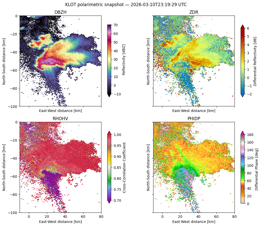
What you’re looking at. This is KLOT (Chicago, IL) at 2026-03-10 23:20 UTC — a strong convective cell south of the radar. A few things to look for:
DBZH over 50 dBZ marks intense precipitation or hail.
The ZDR ↑ + RHOHV ↓ pair (high differential reflectivity, dropped correlation) flags mixed-phase hydrometeors — likely melting or wet hail near the leading edge.
The PHIDP gradient across the storm core scales with rain-path integrated water and is what powers polarimetric rainfall-rate algorithms.
The same five-step pattern — connect → load → slice → georeference → plot — works for any timestamp, any VCP, any KLOT scan in the archive.
Where to next#
Want to reproduce a published figure? → Notebook 2 — QVP comparison reproduces Ryzhkov et al. (2016) Fig. 4 and asserts numerical equivalence between the traditional file-based path and the ARCO streaming path.
Want to estimate rainfall accumulation? → Notebook 3 — QPE scaling applies the Marshall–Palmer Z–R relation live for one day, with cluster-recommended templates for 7-day / 30-day / 6-month windows.
Want to query a different radar or event?
→ The quickstart shows the 5-line connection pattern. Swap "KLOT" for "KVNX" (Oklahoma) to point at a different archive — more radars are added to nexrad-arco as they’re processed.
Want to understand the data model? → About covers the DataTree / Icechunk / Zarr stack and the AtmoScale parent platform. Glossary defines every radar acronym in one place.
Cite this work: Ladino-Rincón, A., et al. (2026). Radar DataTree: A FAIR and Cloud-Native Framework for Scalable Weather Radar Archives. (Manuscript in preparation.) Earlier preprint: arXiv:2510.24943, doi:10.48550/arXiv.2510.24943.