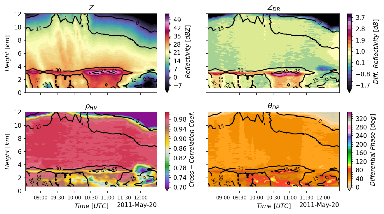
Figure 4 of Ryzhkov et al. (2016) — time-height QVP cross-sections of \(Z\), \(Z_{DR}\), \(\rho_{HV}\), and \(\Phi_{DP}\) for the May 20, 2011 KVNX MCS. This is the figure the notebook reproduces.

QVP Analysis: Traditional vs ARCO Workflows

This notebook reproduces Figure 4 from Ryzhkov et al. (2016) two ways — the traditional file-based workflow and the Analysis-Ready Cloud-Optimized (ARCO) path on s3://nexrad-arco/KVNX — then asserts the results agree to floating-point precision so the speedup is honest rather than apples-to-oranges.

Scientific goal: compute Quasi-Vertical Profiles of \(Z\), \(Z_{DR}\), \(\rho_{HV}\), and \(\Phi_{DP}\) for the May 20, 2011 MCS observed by KVNX during MC3E.

TL;DR

Reproduce Ryzhkov et al. (2016) Fig. 4 in ~5 seconds on a laptop — 60× faster, 22× less RAM than the traditional workflow that downloads and decodes 55 NEXRAD Level II files. The notebook computes the QVP both ways and asserts numerical equivalence between them, so the speedup isn’t a different result — it’s the same result, faster.

---

Prerequisites

This notebook assumes familiarity with the basics covered in Notebook 1 — Open NEXRAD radar archives in 5 lines with radar-datatree:

• Connecting to cloud storage with Icechunk

• Opening a DataTree with engine="rustytree"

• Time-based selection with .sel()

If you’re new to radar-datatree, start there first.

What is a Quasi-Vertical Profile (QVP)?

A Quasi-Vertical Profile (QVP) averages a polarimetric radar variable over all 360° of azimuth at a fixed high elevation (here, 19.5°), collapsing it into a time-height view of the column above the radar:

\[\text{QVP}(r, t) = \frac{1}{N_{\theta}} \sum_{\theta=0}^{360°} Z(r, \theta, t)\]

where \(r\) becomes height after the elevation correction, \(\theta\) is azimuth, and \(t\) is time.

This lets you watch the melting layer, dendritic growth zones, and aggregation signatures evolve through a storm — the killer use case Ryzhkov et al. (2016) introduce. The hero figure at the top is exactly what we’ll reproduce.

Study Parameters

We’ll analyze an expanded time window to capture more storm evolution:

• Radar: KVNX (Vance Air Force Base, Oklahoma)

• Date: May 20, 2011 (MC3E field campaign)

• Time Window: 08:30 - 12:30 UTC (4 hours)

• Elevation: 19.5° (highest WSR-88D elevation, sweep_16)

• Variables: DBZH, ZDR, RHOHV, PHIDP

import sys
import time
import tracemalloc  # For memory tracking
import warnings
from pathlib import Path

# Suppress FutureWarning from xradar/xarray
warnings.filterwarnings("ignore", category=FutureWarning)

# Ensure demo_functions is importable when sphinx-build runs from docs/.
sys.path.insert(0, str(Path("../notebooks").resolve()))

import cmweather  # noqa: F401
import icechunk as ic
import matplotlib.pyplot as plt
import numpy as np
import xarray as xr
from demo_functions import (
    assert_qvp_equivalence,
    calculate_chunk_metrics,
    compute_qvp,
    get_repo_config,
    list_nexrad_files_with_sizes,
    nexrad_download_with_size,
    plot_workflow_comparison,
    print_arco_summary,
    print_chunk_analysis,
    print_traditional_summary,
    print_workflow_comparison,
    ryzhkov_figure,
)

# Study parameters - expanded time window (4 hours)
RADAR = "KVNX"
START_TIME = "2011-05-20 08:30"
END_TIME = "2011-05-20 12:30"
VARIABLES = ["DBZH", "ZDR", "RHOHV", "PHIDP"]
# 19.5° elevation, the angle Ryzhkov et al. (2016) use for QVPs. Both
# the file-based loop below and the ARCO path target this exact sweep
# so they're guaranteed to operate on identical underlying scans.
SELECTED_SWEEP = "sweep_16"

# Metrics collection
metrics = {"traditional": {}, "arco": {}}

---

Approach 1 — Traditional file-based workflow

Discover the files, download each compressed Level II, decode it, extract the 19.5° sweep, concatenate the per-file sweeps along time, compute QVPs. Every stage blocks the next; nothing streams. This is the work the cloud-native path eliminates.

# List all NEXRAD files with actual sizes from AWS S3 using fsspec
t0 = time.time()
nexrad_files = list_nexrad_files_with_sizes(
    radar=RADAR, start_time=START_TIME, end_time=END_TIME
)
metrics["traditional"]["discovery_time"] = time.time() - t0
metrics["traditional"]["n_files"] = len(nexrad_files)
metrics["traditional"]["total_size_bytes"] = sum(f["size"] for f in nexrad_files)
metrics["traditional"]["total_size_mb"] = metrics["traditional"]["total_size_bytes"] / (
    1024 * 1024
)

print(f"Found {len(nexrad_files)} files in the time range")
print(
    f"First file: {nexrad_files[0]['path'].split('/')[-1]} ({nexrad_files[0]['size'] / 1e6:.1f} MB)"
)
print(
    f"Last file:  {nexrad_files[-1]['path'].split('/')[-1]} ({nexrad_files[-1]['size'] / 1e6:.1f} MB)"
)
print(f"\nTotal data volume: {metrics['traditional']['total_size_mb']:.1f} MB")
print(f"Discovery time: {metrics['traditional']['discovery_time']:.2f}s")

Found 55 files in the time range
First file: KVNX20110520_083314_V06.gz (15.0 MB)
Last file:  KVNX20110520_122911_V06.gz (14.0 MB)

Total data volume: 808.9 MB
Discovery time: 0.47s

# Download every file, decode it, extract SELECTED_SWEEP, hold the sweep
# datasets in RAM for later concat. tracemalloc captures the peak — the
# "22× less RAM" claim downstream is grounded in this measurement.
t0 = time.time()
tracemalloc.start()

sweep_datasets = []
download_times = []
bytes_downloaded = 0

for file_info in nexrad_files:
    t_download = time.time()
    dtree_single, size_bytes = nexrad_download_with_size(file_info["path"])
    download_times.append(time.time() - t_download)
    bytes_downloaded += size_bytes

    # KeyError here is intentional — silently averaging across the wrong
    # elevation would corrupt the QVP without anyone noticing.
    ds = dtree_single[SELECTED_SWEEP].ds.load()
    sweep_time = ds.time.values[0]
    ds = ds.expand_dims({"vcp_time": [sweep_time]})
    sweep_datasets.append(ds)

current_mem, peak_mem = tracemalloc.get_traced_memory()
tracemalloc.stop()

metrics["traditional"]["total_time"] = time.time() - t0
metrics["traditional"]["avg_download_time"] = np.mean(download_times)
metrics["traditional"]["files_processed"] = len(sweep_datasets)
metrics["traditional"]["bytes_downloaded"] = bytes_downloaded
metrics["traditional"]["peak_memory_mb"] = peak_mem / 1e6
metrics["traditional"]["final_memory_mb"] = current_mem / 1e6

print(
    f"Downloaded {len(sweep_datasets)} files · "
    f"{bytes_downloaded / 1e6:.0f} MB compressed · "
    f"peak {peak_mem / 1e6:.0f} MB RAM · "
    f"{metrics['traditional']['total_time']:.1f}s total"
)

Downloaded 55 files · 848 MB compressed · peak 3097 MB RAM · 271.6s total

# Concatenate the per-file sweeps, then compute QVPs with the same helper
# the ARCO path uses below. Identical transforms on both sides means the
# results can be compared value-for-value (see the equivalence assertion).
t0_concat = time.time()
tracemalloc.start()

ds_traditional = xr.concat(sweep_datasets, dim="vcp_time")
concat_time = time.time() - t0_concat

t0_qvp = time.time()
qvp_traditional = {
    var: compute_qvp(ds_traditional, var=var)
    for var in VARIABLES
    if var in ds_traditional.data_vars
}
qvp_compute_time = time.time() - t0_qvp

_, peak_mem = tracemalloc.get_traced_memory()
tracemalloc.stop()

metrics["traditional"]["concat_time"] = concat_time
metrics["traditional"]["qvp_compute_time"] = qvp_compute_time
metrics["traditional"]["concat_peak_memory_mb"] = peak_mem / 1e6
metrics["traditional"]["total_workflow_time"] = (
    metrics["traditional"]["total_time"] + concat_time + qvp_compute_time
)

print_traditional_summary(metrics, ds_traditional)

============================================================
TRADITIONAL WORKFLOW - ACTUAL COSTS (ALL FILES)
============================================================
Files processed:               55
Download + decode time:        271.6s
Concatenation time:            1.75s
QVP computation time:          1.86s
TOTAL WORKFLOW TIME:           275.2s (4.6 min)
------------------------------------------------------------
Network transfer (compressed): 808.9 MB
Peak RAM (download phase):     3097 MB
Peak RAM (concat phase):       5793 MB
============================================================

Concatenated dataset shape:
  Time steps: 55
  Azimuth: 2383
  Range: 460
  Variables: ['DBZH', 'VRADH', 'WRADH', 'ZDR', 'PHIDP', 'RHOHV']...

---

Approach 2 — ARCO streaming

Open the Icechunk repository (metadata only), navigate to the sweep we want, slice the 4-hour window on the native vcp_time dimension. No file iteration, no decoding. Chunks stream on demand only when .compute() is called below.

%%time
t0 = time.time()

# Configure S3-compatible storage (OSN)
storage = ic.s3_storage(
    bucket="nexrad-arco",
    prefix="KVNX",
    endpoint_url="https://umn1.osn.mghpcc.org",
    anonymous=True,
    force_path_style=True,
    region="us-east-1",
)

# Connect to repository with optimized config
repo_config = get_repo_config()
repo = ic.Repository.open(storage, config=repo_config)
session = repo.readonly_session("main")

metrics["arco"]["connect_time"] = time.time() - t0
print(f"Connected to Icechunk repository in {metrics['arco']['connect_time']:.2f}s")

Connected to Icechunk repository in 0.63s
CPU times: user 50.4 ms, sys: 6.02 ms, total: 56.4 ms
Wall time: 626 ms

Open the radar datatree using xarray.

%%time
t0 = time.time()

# Open only the sweep we need across all VCPs. The `/*/sweep_16` glob
# trims the tree from "every VCP × every sweep" down to just SELECTED_SWEEP
# (the 19.5° elevation Ryzhkov et al. 2016 use for QVPs). See
# Notebook 1's "Sweep_0 from every VCP" section for the same pattern.
dtree = xr.open_datatree(
    session.store,
    engine="rustytree",
    group=f"/*/{SELECTED_SWEEP}",
    chunks={},
)

metrics["arco"]["open_datatree_time"] = time.time() - t0
print(f"Opened DataTree in {metrics['arco']['open_datatree_time']:.2f}s")

Opened DataTree in 0.69s
CPU times: user 146 ms, sys: 34 ms, total: 180 ms
Wall time: 692 ms

dtree

<xarray.DataTree>
Group: /
├── Group: /VCP-12
│   │   Dimensions:        (vcp_time: 3577)
│   │   Coordinates:
│   │     * vcp_time       (vcp_time) datetime64[ns] 29kB 2011-04-08T22:31:19.547000 ...
│   │       altitude       int64 8B ...
│   │       latitude       float64 8B ...
│   │       longitude      float64 8B ...
│   │   Data variables:
│   │       volume_number  (vcp_time) float64 29kB dask.array<chunksize=(1,), meta=np.ndarray>
│   │   Attributes:
│   │       Conventions:  Cf/Radial instrument_parameters radar_parameters
│   │       attribution:  NOAA NEXRAD Level 2 data processed by Atmoscale from NOAA O...
│   │       dataset_id:   nexrad-arco-kvnx
│   │       institution:  NOAA National Weather Service
│   │       source:       WSR-88D S-band weather radar
│   │       time_domain:  2026-04-27 to Present
│   │       title:        NEXRAD ARCO - KVNX
│   │       version:      2.1
│   └── Group: /VCP-12/sweep_16
│           Dimensions:              (vcp_time: 3577, azimuth: 360, range: 460)
│           Coordinates:
│             * azimuth              (azimuth) float64 3kB 0.5 1.5 2.5 ... 357.5 358.5 359.5
│               elevation            (azimuth) float64 3kB dask.array<chunksize=(360,), meta=np.ndarray>
│               time                 (vcp_time, azimuth) datetime64[ns] 10MB dask.array<chunksize=(1, 360), meta=np.ndarray>
│             * range                (range) float32 2kB 2.125e+03 2.375e+03 ... 1.169e+05
│           Data variables:
│               CCORH                (vcp_time, azimuth, range) float32 2GB dask.array<chunksize=(1, 360, 460), meta=np.ndarray>
│               DBZH                 (vcp_time, azimuth, range) float32 2GB dask.array<chunksize=(1, 360, 460), meta=np.ndarray>
│               PHIDP                (vcp_time, azimuth, range) float32 2GB dask.array<chunksize=(1, 360, 460), meta=np.ndarray>
│               RHOHV                (vcp_time, azimuth, range) float32 2GB dask.array<chunksize=(1, 360, 460), meta=np.ndarray>
│               VRADH                (vcp_time, azimuth, range) float32 2GB dask.array<chunksize=(1, 360, 460), meta=np.ndarray>
│               WRADH                (vcp_time, azimuth, range) float32 2GB dask.array<chunksize=(1, 360, 460), meta=np.ndarray>
│               ZDR                  (vcp_time, azimuth, range) float32 2GB dask.array<chunksize=(1, 360, 460), meta=np.ndarray>
│               ray_elevation_angle  (vcp_time, azimuth) float64 10MB dask.array<chunksize=(1, 360), meta=np.ndarray>
│               sweep_fixed_angle    (vcp_time) float32 14kB dask.array<chunksize=(1,), meta=np.ndarray>
│               sweep_number         (vcp_time) float32 14kB dask.array<chunksize=(1,), meta=np.ndarray>
├── Group: /VCP-121
│   │   Dimensions:        (vcp_time: 1)
│   │   Coordinates:
│   │     * vcp_time       (vcp_time) datetime64[ns] 8B 2011-08-06T03:42:31.495000
│   │       altitude       int64 8B ...
│   │       latitude       float64 8B ...
│   │       longitude      float64 8B ...
│   │   Data variables:
│   │       volume_number  (vcp_time) float64 8B dask.array<chunksize=(1,), meta=np.ndarray>
│   │   Attributes:
│   │       Conventions:  Cf/Radial instrument_parameters radar_parameters
│   │       attribution:  NOAA NEXRAD Level 2 data processed by Atmoscale from NOAA O...
│   │       dataset_id:   nexrad-arco-kvnx
│   │       institution:  NOAA National Weather Service
│   │       source:       WSR-88D S-band weather radar
│   │       time_domain:  2026-04-27 to Present
│   │       title:        NEXRAD ARCO - KVNX
│   │       version:      2.1
│   └── Group: /VCP-121/sweep_16
│           Dimensions:              (vcp_time: 1, azimuth: 360, range: 924)
│           Coordinates:
│             * azimuth              (azimuth) float64 3kB 0.5 1.5 2.5 ... 357.5 358.5 359.5
│               elevation            (azimuth) float64 3kB dask.array<chunksize=(360,), meta=np.ndarray>
│               time                 (vcp_time, azimuth) datetime64[ns] 3kB dask.array<chunksize=(1, 360), meta=np.ndarray>
│             * range                (range) float32 4kB 2.125e+03 2.375e+03 ... 2.329e+05
│           Data variables:
│               DBZH                 (vcp_time, azimuth, range) float32 1MB dask.array<chunksize=(1, 360, 924), meta=np.ndarray>
│               PHIDP                (vcp_time, azimuth, range) float32 1MB dask.array<chunksize=(1, 360, 924), meta=np.ndarray>
│               RHOHV                (vcp_time, azimuth, range) float32 1MB dask.array<chunksize=(1, 360, 924), meta=np.ndarray>
│               VRADH                (vcp_time, azimuth, range) float32 1MB dask.array<chunksize=(1, 360, 924), meta=np.ndarray>
│               WRADH                (vcp_time, azimuth, range) float32 1MB dask.array<chunksize=(1, 360, 924), meta=np.ndarray>
│               ZDR                  (vcp_time, azimuth, range) float32 1MB dask.array<chunksize=(1, 360, 924), meta=np.ndarray>
│               ray_elevation_angle  (vcp_time, azimuth) float64 3kB dask.array<chunksize=(1, 360), meta=np.ndarray>
│               sweep_fixed_angle    (vcp_time) float32 4B dask.array<chunksize=(1,), meta=np.ndarray>
│               sweep_number         (vcp_time) float32 4B dask.array<chunksize=(1,), meta=np.ndarray>
└── Group: /VCP-212
    │   Dimensions:        (vcp_time: 748)
    │   Coordinates:
    │     * vcp_time       (vcp_time) datetime64[ns] 6kB 2011-05-20T19:19:02.487000 ....
    │       altitude       int64 8B ...
    │       latitude       float64 8B ...
    │       longitude      float64 8B ...
    │   Data variables:
    │       volume_number  (vcp_time) float64 6kB dask.array<chunksize=(1,), meta=np.ndarray>
    │   Attributes:
    │       Conventions:  Cf/Radial instrument_parameters radar_parameters
    │       attribution:  NOAA NEXRAD Level 2 data processed by Atmoscale from NOAA O...
    │       dataset_id:   nexrad-arco-kvnx
    │       institution:  NOAA National Weather Service
    │       source:       WSR-88D S-band weather radar
    │       time_domain:  2026-04-27 to Present
    │       title:        NEXRAD ARCO - KVNX
    │       version:      2.1
    └── Group: /VCP-212/sweep_16
            Dimensions:              (vcp_time: 748, azimuth: 360, range: 460)
            Coordinates:
              * azimuth              (azimuth) float64 3kB 0.5 1.5 2.5 ... 357.5 358.5 359.5
                elevation            (azimuth) float64 3kB dask.array<chunksize=(360,), meta=np.ndarray>
                time                 (vcp_time, azimuth) datetime64[ns] 2MB dask.array<chunksize=(1, 360), meta=np.ndarray>
              * range                (range) float32 2kB 2.125e+03 2.375e+03 ... 1.169e+05
            Data variables:
                CCORH                (vcp_time, azimuth, range) float32 495MB dask.array<chunksize=(1, 360, 460), meta=np.ndarray>
                DBZH                 (vcp_time, azimuth, range) float32 495MB dask.array<chunksize=(1, 360, 460), meta=np.ndarray>
                PHIDP                (vcp_time, azimuth, range) float32 495MB dask.array<chunksize=(1, 360, 460), meta=np.ndarray>
                RHOHV                (vcp_time, azimuth, range) float32 495MB dask.array<chunksize=(1, 360, 460), meta=np.ndarray>
                VRADH                (vcp_time, azimuth, range) float32 495MB dask.array<chunksize=(1, 360, 460), meta=np.ndarray>
                WRADH                (vcp_time, azimuth, range) float32 495MB dask.array<chunksize=(1, 360, 460), meta=np.ndarray>
                ZDR                  (vcp_time, azimuth, range) float32 495MB dask.array<chunksize=(1, 360, 460), meta=np.ndarray>
                ray_elevation_angle  (vcp_time, azimuth) float64 2MB dask.array<chunksize=(1, 360), meta=np.ndarray>
                sweep_fixed_angle    (vcp_time) float32 3kB dask.array<chunksize=(1,), meta=np.ndarray>
                sweep_number         (vcp_time) float32 3kB dask.array<chunksize=(1,), meta=np.ndarray>

xarray.DataTree

• /VCP-12(27)

  • /VCP-12/sweep_16(14)

    • Dimensions:
      • vcp_time: 3577
      • azimuth: 360
      • range: 460
    • Coordinates: (4)
      • azimuth
        (azimuth)
        float64
        0.5 1.5 2.5 ... 357.5 358.5 359.5

        array([  0.5,   1.5,   2.5, ..., 357.5, 358.5, 359.5], shape=(360,))

      • elevation
        (azimuth)
        float64
        dask.array<chunksize=(360,), meta=np.ndarray>

        axis :

        radial_elevation_coordinate

        long_name :

        elevation_angle_from_horizontal_plane

        standard_name :

        ray_elevation_angle

        units :

        degrees

        Array Chunk Bytes 2.81 kiB 2.81 kiB Shape (360,) (360,) Dask graph 1 chunks in 2 graph layers Data type float64 numpy.ndarray

      • time
        (vcp_time, azimuth)
        datetime64[ns]
        dask.array<chunksize=(1, 360), meta=np.ndarray>

        standard_name :

        time

        Array Chunk Bytes 9.82 MiB 2.81 kiB Shape (3577, 360) (1, 360) Dask graph 3577 chunks in 2 graph layers Data type datetime64[ns] numpy.ndarray

      • range
        (range)
        float32
        2.125e+03 2.375e+03 ... 1.169e+05

        axis :

        radial_range_coordinate

        long_name :

        range_to_measurement_volume

        meters_between_gates :

        250.0

        meters_to_center_of_first_gate :

        2125.0

        spacing_is_constant :

        true

        standard_name :

        projection_range_coordinate

        units :

        meters

        array([  2125.,   2375.,   2625., ..., 116375., 116625., 116875.],shape=(460,), dtype=float32)

    • Data variables: (10)
      • CCORH
        (vcp_time, azimuth, range)
        float32
        dask.array<chunksize=(1, 360, 460), meta=np.ndarray>

        long_name :

        Clutter Correction H

        standard_name :

        clutter_correction_h

        units :

        unitless

        Array Chunk Bytes 2.21 GiB 646.88 kiB Shape (3577, 360, 460) (1, 360, 460) Dask graph 3577 chunks in 2 graph layers Data type float32 numpy.ndarray

      • DBZH
        (vcp_time, azimuth, range)
        float32
        dask.array<chunksize=(1, 360, 460), meta=np.ndarray>

        long_name :

        Equivalent reflectivity factor H

        standard_name :

        radar_equivalent_reflectivity_factor_h

        units :

        dBZ

        Array Chunk Bytes 2.21 GiB 646.88 kiB Shape (3577, 360, 460) (1, 360, 460) Dask graph 3577 chunks in 2 graph layers Data type float32 numpy.ndarray

      • PHIDP
        (vcp_time, azimuth, range)
        float32
        dask.array<chunksize=(1, 360, 460), meta=np.ndarray>

        long_name :

        Differential phase HV

        standard_name :

        radar_differential_phase_hv

        units :

        degrees

        Array Chunk Bytes 2.21 GiB 646.88 kiB Shape (3577, 360, 460) (1, 360, 460) Dask graph 3577 chunks in 2 graph layers Data type float32 numpy.ndarray

      • RHOHV
        (vcp_time, azimuth, range)
        float32
        dask.array<chunksize=(1, 360, 460), meta=np.ndarray>

        long_name :

        Correlation coefficient HV

        standard_name :

        radar_correlation_coefficient_hv

        units :

        unitless

        Array Chunk Bytes 2.21 GiB 646.88 kiB Shape (3577, 360, 460) (1, 360, 460) Dask graph 3577 chunks in 2 graph layers Data type float32 numpy.ndarray

      • VRADH
        (vcp_time, azimuth, range)
        float32
        dask.array<chunksize=(1, 360, 460), meta=np.ndarray>

        long_name :

        Radial velocity H

        standard_name :

        radial_velocity_of_scatterers_away_from_instrument

        units :

        m/s

        Array Chunk Bytes 2.21 GiB 646.88 kiB Shape (3577, 360, 460) (1, 360, 460) Dask graph 3577 chunks in 2 graph layers Data type float32 numpy.ndarray

      • WRADH
        (vcp_time, azimuth, range)
        float32
        dask.array<chunksize=(1, 360, 460), meta=np.ndarray>

        long_name :

        Doppler spectrum width H

        standard_name :

        radar_spectrum_width

        units :

        m/s

        Array Chunk Bytes 2.21 GiB 646.88 kiB Shape (3577, 360, 460) (1, 360, 460) Dask graph 3577 chunks in 2 graph layers Data type float32 numpy.ndarray

      • ZDR
        (vcp_time, azimuth, range)
        float32
        dask.array<chunksize=(1, 360, 460), meta=np.ndarray>

        long_name :

        Log differential reflectivity H/V

        standard_name :

        radar_differential_reflectivity_hv

        units :

        dB

        Array Chunk Bytes 2.21 GiB 646.88 kiB Shape (3577, 360, 460) (1, 360, 460) Dask graph 3577 chunks in 2 graph layers Data type float32 numpy.ndarray

      • ray_elevation_angle
        (vcp_time, azimuth)
        float64
        dask.array<chunksize=(1, 360), meta=np.ndarray>

        axis :

        radial_elevation_coordinate

        long_name :

        elevation_angle_from_horizontal_plane

        standard_name :

        ray_elevation_angle

        units :

        degrees

        Array Chunk Bytes 9.82 MiB 2.81 kiB Shape (3577, 360) (1, 360) Dask graph 3577 chunks in 2 graph layers Data type float64 numpy.ndarray

      • sweep_fixed_angle
        (vcp_time)
        float32
        dask.array<chunksize=(1,), meta=np.ndarray>

        Array Chunk Bytes 13.97 kiB 4 B Shape (3577,) (1,) Dask graph 3577 chunks in 2 graph layers Data type float32 numpy.ndarray

      • sweep_number
        (vcp_time)
        float32
        dask.array<chunksize=(1,), meta=np.ndarray>

        Array Chunk Bytes 13.97 kiB 4 B Shape (3577,) (1,) Dask graph 3577 chunks in 2 graph layers Data type float32 numpy.ndarray

  • Dimensions:
    • vcp_time: 3577
  • Coordinates: (4)
    • vcp_time
      (vcp_time)
      datetime64[ns]
      2011-04-08T22:31:19.547000 ... 2...

      axis :

      T

      description :

      Volume Coverage Pattern time since start of volume scan

      long_name :

      time of volume coverage pattern scan

      standard_name :

      time

      array(['2011-04-08T22:31:19.547000000', '2011-04-08T22:35:40.841000000','2011-04-08T22:40:01.859000000', ..., '2011-09-18T11:43:51.817000000','2011-09-18T11:48:11.937000000', '2011-09-18T11:52:32.427000000'],shape=(3577,), dtype='datetime64[ns]')

    • altitude
      ()
      int64
      ...

      [1 values with dtype=int64]

    • latitude
      ()
      float64
      ...

      [1 values with dtype=float64]

    • longitude
      ()
      float64
      ...

      [1 values with dtype=float64]

  • Data variables: (1)
    • volume_number
      (vcp_time)
      float64
      dask.array<chunksize=(1,), meta=np.ndarray>

      Array Chunk Bytes 27.95 kiB 8 B Shape (3577,) (1,) Dask graph 3577 chunks in 2 graph layers Data type float64 numpy.ndarray

  • Attributes: (8)

    Conventions :

    Cf/Radial instrument_parameters radar_parameters

    attribution :

    NOAA NEXRAD Level 2 data processed by Atmoscale from NOAA Open Data Dissemination archives.

    dataset_id :

    nexrad-arco-kvnx

    institution :

    NOAA National Weather Service

    source :

    WSR-88D S-band weather radar

    time_domain :

    2026-04-27 to Present

    title :

    NEXRAD ARCO - KVNX

    version :

    2.1

  /VCP-121(26)

  • /VCP-121/sweep_16(13)

    • Dimensions:
      • vcp_time: 1
      • azimuth: 360
      • range: 924
    • Coordinates: (4)
      • azimuth
        (azimuth)
        float64
        0.5 1.5 2.5 ... 357.5 358.5 359.5

        array([  0.5,   1.5,   2.5, ..., 357.5, 358.5, 359.5], shape=(360,))

      • elevation
        (azimuth)
        float64
        dask.array<chunksize=(360,), meta=np.ndarray>

        axis :

        radial_elevation_coordinate

        long_name :

        elevation_angle_from_horizontal_plane

        standard_name :

        ray_elevation_angle

        units :

        degrees

        Array Chunk Bytes 2.81 kiB 2.81 kiB Shape (360,) (360,) Dask graph 1 chunks in 2 graph layers Data type float64 numpy.ndarray

      • time
        (vcp_time, azimuth)
        datetime64[ns]
        dask.array<chunksize=(1, 360), meta=np.ndarray>

        standard_name :

        time

        Array Chunk Bytes 2.81 kiB 2.81 kiB Shape (1, 360) (1, 360) Dask graph 1 chunks in 2 graph layers Data type datetime64[ns] numpy.ndarray

      • range
        (range)
        float32
        2.125e+03 2.375e+03 ... 2.329e+05

        axis :

        radial_range_coordinate

        long_name :

        range_to_measurement_volume

        meters_between_gates :

        250.0

        meters_to_center_of_first_gate :

        2125.0

        spacing_is_constant :

        true

        standard_name :

        projection_range_coordinate

        units :

        meters

        array([  2125.,   2375.,   2625., ..., 232375., 232625., 232875.],shape=(924,), dtype=float32)

    • Data variables: (9)
      • DBZH
        (vcp_time, azimuth, range)
        float32
        dask.array<chunksize=(1, 360, 924), meta=np.ndarray>

        long_name :

        Equivalent reflectivity factor H

        standard_name :

        radar_equivalent_reflectivity_factor_h

        units :

        dBZ

        Array Chunk Bytes 1.27 MiB 1.27 MiB Shape (1, 360, 924) (1, 360, 924) Dask graph 1 chunks in 2 graph layers Data type float32 numpy.ndarray

      • PHIDP
        (vcp_time, azimuth, range)
        float32
        dask.array<chunksize=(1, 360, 924), meta=np.ndarray>

        long_name :

        Differential phase HV

        standard_name :

        radar_differential_phase_hv

        units :

        degrees

        Array Chunk Bytes 1.27 MiB 1.27 MiB Shape (1, 360, 924) (1, 360, 924) Dask graph 1 chunks in 2 graph layers Data type float32 numpy.ndarray

      • RHOHV
        (vcp_time, azimuth, range)
        float32
        dask.array<chunksize=(1, 360, 924), meta=np.ndarray>

        long_name :

        Correlation coefficient HV

        standard_name :

        radar_correlation_coefficient_hv

        units :

        unitless

        Array Chunk Bytes 1.27 MiB 1.27 MiB Shape (1, 360, 924) (1, 360, 924) Dask graph 1 chunks in 2 graph layers Data type float32 numpy.ndarray

      • VRADH
        (vcp_time, azimuth, range)
        float32
        dask.array<chunksize=(1, 360, 924), meta=np.ndarray>

        long_name :

        Radial velocity H

        standard_name :

        radial_velocity_of_scatterers_away_from_instrument

        units :

        m/s

        Array Chunk Bytes 1.27 MiB 1.27 MiB Shape (1, 360, 924) (1, 360, 924) Dask graph 1 chunks in 2 graph layers Data type float32 numpy.ndarray

      • WRADH
        (vcp_time, azimuth, range)
        float32
        dask.array<chunksize=(1, 360, 924), meta=np.ndarray>

        long_name :

        Doppler spectrum width H

        standard_name :

        radar_spectrum_width

        units :

        m/s

        Array Chunk Bytes 1.27 MiB 1.27 MiB Shape (1, 360, 924) (1, 360, 924) Dask graph 1 chunks in 2 graph layers Data type float32 numpy.ndarray

      • ZDR
        (vcp_time, azimuth, range)
        float32
        dask.array<chunksize=(1, 360, 924), meta=np.ndarray>

        long_name :

        Log differential reflectivity H/V

        standard_name :

        radar_differential_reflectivity_hv

        units :

        dB

        Array Chunk Bytes 1.27 MiB 1.27 MiB Shape (1, 360, 924) (1, 360, 924) Dask graph 1 chunks in 2 graph layers Data type float32 numpy.ndarray

      • ray_elevation_angle
        (vcp_time, azimuth)
        float64
        dask.array<chunksize=(1, 360), meta=np.ndarray>

        axis :

        radial_elevation_coordinate

        long_name :

        elevation_angle_from_horizontal_plane

        standard_name :

        ray_elevation_angle

        units :

        degrees

        Array Chunk Bytes 2.81 kiB 2.81 kiB Shape (1, 360) (1, 360) Dask graph 1 chunks in 2 graph layers Data type float64 numpy.ndarray

      • sweep_fixed_angle
        (vcp_time)
        float32
        dask.array<chunksize=(1,), meta=np.ndarray>

        Array Chunk Bytes 4 B 4 B Shape (1,) (1,) Dask graph 1 chunks in 2 graph layers Data type float32 numpy.ndarray

      • sweep_number
        (vcp_time)
        float32
        dask.array<chunksize=(1,), meta=np.ndarray>

        Array Chunk Bytes 4 B 4 B Shape (1,) (1,) Dask graph 1 chunks in 2 graph layers Data type float32 numpy.ndarray

  • Dimensions:
    • vcp_time: 1
  • Coordinates: (4)
    • vcp_time
      (vcp_time)
      datetime64[ns]
      2011-08-06T03:42:31.495000

      axis :

      T

      description :

      Volume Coverage Pattern time since start of volume scan

      long_name :

      time of volume coverage pattern scan

      standard_name :

      time

      array(['2011-08-06T03:42:31.495000000'], dtype='datetime64[ns]')

    • altitude
      ()
      int64
      ...

      [1 values with dtype=int64]

    • latitude
      ()
      float64
      ...

      [1 values with dtype=float64]

    • longitude
      ()
      float64
      ...

      [1 values with dtype=float64]

  • Data variables: (1)
    • volume_number
      (vcp_time)
      float64
      dask.array<chunksize=(1,), meta=np.ndarray>

      Array Chunk Bytes 8 B 8 B Shape (1,) (1,) Dask graph 1 chunks in 2 graph layers Data type float64 numpy.ndarray

  • Attributes: (8)

    Conventions :

    Cf/Radial instrument_parameters radar_parameters

    attribution :

    NOAA NEXRAD Level 2 data processed by Atmoscale from NOAA Open Data Dissemination archives.

    dataset_id :

    nexrad-arco-kvnx

    institution :

    NOAA National Weather Service

    source :

    WSR-88D S-band weather radar

    time_domain :

    2026-04-27 to Present

    title :

    NEXRAD ARCO - KVNX

    version :

    2.1

  /VCP-212(27)

  • /VCP-212/sweep_16(14)

    • Dimensions:
      • vcp_time: 748
      • azimuth: 360
      • range: 460
    • Coordinates: (4)
      • azimuth
        (azimuth)
        float64
        0.5 1.5 2.5 ... 357.5 358.5 359.5

        array([  0.5,   1.5,   2.5, ..., 357.5, 358.5, 359.5], shape=(360,))

      • elevation
        (azimuth)
        float64
        dask.array<chunksize=(360,), meta=np.ndarray>

        axis :

        radial_elevation_coordinate

        long_name :

        elevation_angle_from_horizontal_plane

        standard_name :

        ray_elevation_angle

        units :

        degrees

        Array Chunk Bytes 2.81 kiB 2.81 kiB Shape (360,) (360,) Dask graph 1 chunks in 2 graph layers Data type float64 numpy.ndarray

      • time
        (vcp_time, azimuth)
        datetime64[ns]
        dask.array<chunksize=(1, 360), meta=np.ndarray>

        standard_name :

        time

        Array Chunk Bytes 2.05 MiB 2.81 kiB Shape (748, 360) (1, 360) Dask graph 748 chunks in 2 graph layers Data type datetime64[ns] numpy.ndarray

      • range
        (range)
        float32
        2.125e+03 2.375e+03 ... 1.169e+05

        axis :

        radial_range_coordinate

        long_name :

        range_to_measurement_volume

        meters_between_gates :

        250.0

        meters_to_center_of_first_gate :

        2125.0

        spacing_is_constant :

        true

        standard_name :

        projection_range_coordinate

        units :

        meters

        array([  2125.,   2375.,   2625., ..., 116375., 116625., 116875.],shape=(460,), dtype=float32)

    • Data variables: (10)
      • CCORH
        (vcp_time, azimuth, range)
        float32
        dask.array<chunksize=(1, 360, 460), meta=np.ndarray>

        long_name :

        Clutter Correction H

        standard_name :

        clutter_correction_h

        units :

        unitless

        Array Chunk Bytes 472.52 MiB 646.88 kiB Shape (748, 360, 460) (1, 360, 460) Dask graph 748 chunks in 2 graph layers Data type float32 numpy.ndarray

      • DBZH
        (vcp_time, azimuth, range)
        float32
        dask.array<chunksize=(1, 360, 460), meta=np.ndarray>

        long_name :

        Equivalent reflectivity factor H

        standard_name :

        radar_equivalent_reflectivity_factor_h

        units :

        dBZ

        Array Chunk Bytes 472.52 MiB 646.88 kiB Shape (748, 360, 460) (1, 360, 460) Dask graph 748 chunks in 2 graph layers Data type float32 numpy.ndarray

      • PHIDP
        (vcp_time, azimuth, range)
        float32
        dask.array<chunksize=(1, 360, 460), meta=np.ndarray>

        long_name :

        Differential phase HV

        standard_name :

        radar_differential_phase_hv

        units :

        degrees

        Array Chunk Bytes 472.52 MiB 646.88 kiB Shape (748, 360, 460) (1, 360, 460) Dask graph 748 chunks in 2 graph layers Data type float32 numpy.ndarray

      • RHOHV
        (vcp_time, azimuth, range)
        float32
        dask.array<chunksize=(1, 360, 460), meta=np.ndarray>

        long_name :

        Correlation coefficient HV

        standard_name :

        radar_correlation_coefficient_hv

        units :

        unitless

        Array Chunk Bytes 472.52 MiB 646.88 kiB Shape (748, 360, 460) (1, 360, 460) Dask graph 748 chunks in 2 graph layers Data type float32 numpy.ndarray

      • VRADH
        (vcp_time, azimuth, range)
        float32
        dask.array<chunksize=(1, 360, 460), meta=np.ndarray>

        long_name :

        Radial velocity H

        standard_name :

        radial_velocity_of_scatterers_away_from_instrument

        units :

        m/s

        Array Chunk Bytes 472.52 MiB 646.88 kiB Shape (748, 360, 460) (1, 360, 460) Dask graph 748 chunks in 2 graph layers Data type float32 numpy.ndarray

      • WRADH
        (vcp_time, azimuth, range)
        float32
        dask.array<chunksize=(1, 360, 460), meta=np.ndarray>

        long_name :

        Doppler spectrum width H

        standard_name :

        radar_spectrum_width

        units :

        m/s

        Array Chunk Bytes 472.52 MiB 646.88 kiB Shape (748, 360, 460) (1, 360, 460) Dask graph 748 chunks in 2 graph layers Data type float32 numpy.ndarray

      • ZDR
        (vcp_time, azimuth, range)
        float32
        dask.array<chunksize=(1, 360, 460), meta=np.ndarray>

        long_name :

        Log differential reflectivity H/V

        standard_name :

        radar_differential_reflectivity_hv

        units :

        dB

        Array Chunk Bytes 472.52 MiB 646.88 kiB Shape (748, 360, 460) (1, 360, 460) Dask graph 748 chunks in 2 graph layers Data type float32 numpy.ndarray

      • ray_elevation_angle
        (vcp_time, azimuth)
        float64
        dask.array<chunksize=(1, 360), meta=np.ndarray>

        axis :

        radial_elevation_coordinate

        long_name :

        elevation_angle_from_horizontal_plane

        standard_name :

        ray_elevation_angle

        units :

        degrees

        Array Chunk Bytes 2.05 MiB 2.81 kiB Shape (748, 360) (1, 360) Dask graph 748 chunks in 2 graph layers Data type float64 numpy.ndarray

      • sweep_fixed_angle
        (vcp_time)
        float32
        dask.array<chunksize=(1,), meta=np.ndarray>

        Array Chunk Bytes 2.92 kiB 4 B Shape (748,) (1,) Dask graph 748 chunks in 2 graph layers Data type float32 numpy.ndarray

      • sweep_number
        (vcp_time)
        float32
        dask.array<chunksize=(1,), meta=np.ndarray>

        Array Chunk Bytes 2.92 kiB 4 B Shape (748,) (1,) Dask graph 748 chunks in 2 graph layers Data type float32 numpy.ndarray

  • Dimensions:
    • vcp_time: 748
  • Coordinates: (4)
    • vcp_time
      (vcp_time)
      datetime64[ns]
      2011-05-20T19:19:02.487000 ... 2...

      axis :

      T

      description :

      Volume Coverage Pattern time since start of volume scan

      long_name :

      time of volume coverage pattern scan

      standard_name :

      time

      array(['2011-05-20T19:19:02.487000000', '2011-05-20T19:23:43.749000000','2011-05-20T19:28:26.192000000', ..., '2011-08-13T02:05:39.624000000','2011-08-13T02:10:20.078000000', '2011-08-13T02:15:00.456000000'],shape=(748,), dtype='datetime64[ns]')

    • altitude
      ()
      int64
      ...

      [1 values with dtype=int64]

    • latitude
      ()
      float64
      ...

      [1 values with dtype=float64]

    • longitude
      ()
      float64
      ...

      [1 values with dtype=float64]

  • Data variables: (1)
    • volume_number
      (vcp_time)
      float64
      dask.array<chunksize=(1,), meta=np.ndarray>

      Array Chunk Bytes 5.84 kiB 8 B Shape (748,) (1,) Dask graph 748 chunks in 2 graph layers Data type float64 numpy.ndarray

  • Attributes: (8)

    Conventions :

    Cf/Radial instrument_parameters radar_parameters

    attribution :

    NOAA NEXRAD Level 2 data processed by Atmoscale from NOAA Open Data Dissemination archives.

    dataset_id :

    nexrad-arco-kvnx

    institution :

    NOAA National Weather Service

    source :

    WSR-88D S-band weather radar

    time_domain :

    2026-04-27 to Present

    title :

    NEXRAD ARCO - KVNX

    version :

    2.1

list(dtree.children)

['VCP-12', 'VCP-121', 'VCP-212']

Each VCP’s sweep_16 is the 19.5° elevation cut. The QVP-target VCP for the May 2011 KVNX MCS is VCP-12 (precipitation mode); pull its sweep directly:

# Select the 4-hour time window
# With ARCO format, this is a simple slice operation - no file iteration needed
ds_qvp_selected = (
    dtree.sel(vcp_time=slice(START_TIME, END_TIME))
    .prune(drop_size_zero_vars=True)[f"/VCP-12/{SELECTED_SWEEP}"]
    .to_dataset()
)


ds_qvp_selected

<xarray.Dataset> Size: 255MB
Dimensions:              (vcp_time: 55, azimuth: 360, range: 460)
Coordinates:
  * vcp_time             (vcp_time) datetime64[ns] 440B 2011-05-20T08:33:14.1...
  * azimuth              (azimuth) float64 3kB 0.5 1.5 2.5 ... 357.5 358.5 359.5
    elevation            (azimuth) float64 3kB dask.array<chunksize=(360,), meta=np.ndarray>
    time                 (vcp_time, azimuth) datetime64[ns] 158kB dask.array<chunksize=(1, 360), meta=np.ndarray>
  * range                (range) float32 2kB 2.125e+03 2.375e+03 ... 1.169e+05
Data variables:
    CCORH                (vcp_time, azimuth, range) float32 36MB dask.array<chunksize=(1, 360, 460), meta=np.ndarray>
    DBZH                 (vcp_time, azimuth, range) float32 36MB dask.array<chunksize=(1, 360, 460), meta=np.ndarray>
    PHIDP                (vcp_time, azimuth, range) float32 36MB dask.array<chunksize=(1, 360, 460), meta=np.ndarray>
    RHOHV                (vcp_time, azimuth, range) float32 36MB dask.array<chunksize=(1, 360, 460), meta=np.ndarray>
    VRADH                (vcp_time, azimuth, range) float32 36MB dask.array<chunksize=(1, 360, 460), meta=np.ndarray>
    WRADH                (vcp_time, azimuth, range) float32 36MB dask.array<chunksize=(1, 360, 460), meta=np.ndarray>
    ZDR                  (vcp_time, azimuth, range) float32 36MB dask.array<chunksize=(1, 360, 460), meta=np.ndarray>
    ray_elevation_angle  (vcp_time, azimuth) float64 158kB dask.array<chunksize=(1, 360), meta=np.ndarray>
    sweep_fixed_angle    (vcp_time) float32 220B dask.array<chunksize=(1,), meta=np.ndarray>
    sweep_number         (vcp_time) float32 220B dask.array<chunksize=(1,), meta=np.ndarray>

xarray.Dataset

• Dimensions:
  • vcp_time: 55
  • azimuth: 360
  • range: 460
• Coordinates: (5)
  • vcp_time
    (vcp_time)
    datetime64[ns]
    2011-05-20T08:33:14.127000 ... 2...

    axis :

    T

    description :

    Volume Coverage Pattern time since start of volume scan

    long_name :

    time of volume coverage pattern scan

    standard_name :

    time

    array(['2011-05-20T08:33:14.127000000', '2011-05-20T08:37:34.426000000',
           '2011-05-20T08:41:53.574000000', '2011-05-20T08:46:12.952000000',
           '2011-05-20T08:50:33.364000000', '2011-05-20T08:54:53.608000000',
           '2011-05-20T08:59:12.789000000', '2011-05-20T09:03:33.061000000',
           '2011-05-20T09:07:53.203000000', '2011-05-20T09:12:12.400000000',
           '2011-05-20T09:16:32.837000000', '2011-05-20T09:20:52.255000000',
           '2011-05-20T09:27:09.585000000', '2011-05-20T09:31:28.788000000',
           '2011-05-20T09:35:48.134000000', '2011-05-20T09:40:09.521000000',
           '2011-05-20T09:44:29.563000000', '2011-05-20T09:48:49.046000000',
           '2011-05-20T09:53:08.262000000', '2011-05-20T09:57:27.484000000',
           '2011-05-20T10:01:47.882000000', '2011-05-20T10:06:08.216000000',
           '2011-05-20T10:10:28.356000000', '2011-05-20T10:14:47.812000000',
           '2011-05-20T10:19:06.937000000', '2011-05-20T10:23:27.361000000',
           '2011-05-20T10:27:47.763000000', '2011-05-20T10:32:07.679000000',
           '2011-05-20T10:36:28.128000000', '2011-05-20T10:40:47.402000000',
           '2011-05-20T10:45:07.823000000', '2011-05-20T10:49:28.114000000',
           '2011-05-20T10:53:49.401000000', '2011-05-20T10:58:09.725000000',
           '2011-05-20T11:02:30.828000000', '2011-05-20T11:06:51.182000000',
           '2011-05-20T11:11:11.450000000', '2011-05-20T11:15:30.806000000',
           '2011-05-20T11:19:51.130000000', '2011-05-20T11:24:10.404000000',
           '2011-05-20T11:28:30.608000000', '2011-05-20T11:32:51.004000000',
           '2011-05-20T11:37:10.304000000', '2011-05-20T11:41:30.595000000',
           '2011-05-20T11:45:50.924000000', '2011-05-20T11:50:11.097000000',
           '2011-05-20T11:54:31.576000000', '2011-05-20T11:58:51.755000000',
           '2011-05-20T12:03:11.035000000', '2011-05-20T12:07:31.258000000',
           '2011-05-20T12:11:50.592000000', '2011-05-20T12:16:11.898000000',
           '2011-05-20T12:20:30.806000000', '2011-05-20T12:24:52.272000000',
           '2011-05-20T12:29:11.734000000'], dtype='datetime64[ns]')

  • azimuth
    (azimuth)
    float64
    0.5 1.5 2.5 ... 357.5 358.5 359.5

    array([  0.5,   1.5,   2.5, ..., 357.5, 358.5, 359.5], shape=(360,))

  • elevation
    (azimuth)
    float64
    dask.array<chunksize=(360,), meta=np.ndarray>

    axis :

    radial_elevation_coordinate

    long_name :

    elevation_angle_from_horizontal_plane

    standard_name :

    ray_elevation_angle

    units :

    degrees

    Array Chunk Bytes 2.81 kiB 2.81 kiB Shape (360,) (360,) Dask graph 1 chunks in 2 graph layers Data type float64 numpy.ndarray

  • time
    (vcp_time, azimuth)
    datetime64[ns]
    dask.array<chunksize=(1, 360), meta=np.ndarray>

    standard_name :

    time

    Array Chunk Bytes 154.69 kiB 2.81 kiB Shape (55, 360) (1, 360) Dask graph 55 chunks in 3 graph layers Data type datetime64[ns] numpy.ndarray

  • range
    (range)
    float32
    2.125e+03 2.375e+03 ... 1.169e+05

    axis :

    radial_range_coordinate

    long_name :

    range_to_measurement_volume

    meters_between_gates :

    250.0

    meters_to_center_of_first_gate :

    2125.0

    spacing_is_constant :

    true

    standard_name :

    projection_range_coordinate

    units :

    meters

    array([  2125.,   2375.,   2625., ..., 116375., 116625., 116875.],
          shape=(460,), dtype=float32)

• Data variables: (10)
  • CCORH
    (vcp_time, azimuth, range)
    float32
    dask.array<chunksize=(1, 360, 460), meta=np.ndarray>

    long_name :

    Clutter Correction H

    standard_name :

    clutter_correction_h

    units :

    unitless

    Array Chunk Bytes 34.74 MiB 646.88 kiB Shape (55, 360, 460) (1, 360, 460) Dask graph 55 chunks in 3 graph layers Data type float32 numpy.ndarray

  • DBZH
    (vcp_time, azimuth, range)
    float32
    dask.array<chunksize=(1, 360, 460), meta=np.ndarray>

    long_name :

    Equivalent reflectivity factor H

    standard_name :

    radar_equivalent_reflectivity_factor_h

    units :

    dBZ

    Array Chunk Bytes 34.74 MiB 646.88 kiB Shape (55, 360, 460) (1, 360, 460) Dask graph 55 chunks in 3 graph layers Data type float32 numpy.ndarray

  • PHIDP
    (vcp_time, azimuth, range)
    float32
    dask.array<chunksize=(1, 360, 460), meta=np.ndarray>

    long_name :

    Differential phase HV

    standard_name :

    radar_differential_phase_hv

    units :

    degrees

    Array Chunk Bytes 34.74 MiB 646.88 kiB Shape (55, 360, 460) (1, 360, 460) Dask graph 55 chunks in 3 graph layers Data type float32 numpy.ndarray

  • RHOHV
    (vcp_time, azimuth, range)
    float32
    dask.array<chunksize=(1, 360, 460), meta=np.ndarray>

    long_name :

    Correlation coefficient HV

    standard_name :

    radar_correlation_coefficient_hv

    units :

    unitless

    Array Chunk Bytes 34.74 MiB 646.88 kiB Shape (55, 360, 460) (1, 360, 460) Dask graph 55 chunks in 3 graph layers Data type float32 numpy.ndarray

  • VRADH
    (vcp_time, azimuth, range)
    float32
    dask.array<chunksize=(1, 360, 460), meta=np.ndarray>

    long_name :

    Radial velocity H

    standard_name :

    radial_velocity_of_scatterers_away_from_instrument

    units :

    m/s

    Array Chunk Bytes 34.74 MiB 646.88 kiB Shape (55, 360, 460) (1, 360, 460) Dask graph 55 chunks in 3 graph layers Data type float32 numpy.ndarray

  • WRADH
    (vcp_time, azimuth, range)
    float32
    dask.array<chunksize=(1, 360, 460), meta=np.ndarray>

    long_name :

    Doppler spectrum width H

    standard_name :

    radar_spectrum_width

    units :

    m/s

    Array Chunk Bytes 34.74 MiB 646.88 kiB Shape (55, 360, 460) (1, 360, 460) Dask graph 55 chunks in 3 graph layers Data type float32 numpy.ndarray

  • ZDR
    (vcp_time, azimuth, range)
    float32
    dask.array<chunksize=(1, 360, 460), meta=np.ndarray>

    long_name :

    Log differential reflectivity H/V

    standard_name :

    radar_differential_reflectivity_hv

    units :

    dB

    Array Chunk Bytes 34.74 MiB 646.88 kiB Shape (55, 360, 460) (1, 360, 460) Dask graph 55 chunks in 3 graph layers Data type float32 numpy.ndarray

  • ray_elevation_angle
    (vcp_time, azimuth)
    float64
    dask.array<chunksize=(1, 360), meta=np.ndarray>

    axis :

    radial_elevation_coordinate

    long_name :

    elevation_angle_from_horizontal_plane

    standard_name :

    ray_elevation_angle

    units :

    degrees

    Array Chunk Bytes 154.69 kiB 2.81 kiB Shape (55, 360) (1, 360) Dask graph 55 chunks in 3 graph layers Data type float64 numpy.ndarray

  • sweep_fixed_angle
    (vcp_time)
    float32
    dask.array<chunksize=(1,), meta=np.ndarray>

    Array Chunk Bytes 220 B 4 B Shape (55,) (1,) Dask graph 55 chunks in 3 graph layers Data type float32 numpy.ndarray

  • sweep_number
    (vcp_time)
    float32
    dask.array<chunksize=(1,), meta=np.ndarray>

    Array Chunk Bytes 220 B 4 B Shape (55,) (1,) Dask graph 55 chunks in 3 graph layers Data type float32 numpy.ndarray

# Calculate ARCO streaming metrics — data fetched on-demand
n_chunks, arco_bytes, chunk_details = calculate_chunk_metrics(
    ds_qvp_selected, VARIABLES
)

# 17 sweeps per VCP-12 NEXRAD Level II volume; the QVP uses the highest one
# (sweep_16 ≈ 19.5°), so traditional downloads everything and discards 16/17.
N_TOTAL_SWEEPS = 17

# Side effect: stashes uncompressed_mb on both branches + chunk_details under
# metrics so print_workflow_comparison reads from a single source of truth.
print_chunk_analysis(
    metrics,
    chunk_details,
    n_chunks,
    arco_bytes,
    selected_sweep=SELECTED_SWEEP,
    n_total_sweeps=N_TOTAL_SWEEPS,
)

metrics["arco"]["n_chunks"] = n_chunks

DATA ACCESS ANALYSIS:
======================================================================

ARCO - Selective Chunk Streaming (sweep_16, 4 variables):
----------------------------------------------------------------------
  NOTE: No compression in this ARCO dataset - network = data size

  DBZH: 55 chunks × 0.66 MB = 36.4 MB
  ZDR: 55 chunks × 0.66 MB = 36.4 MB
  RHOHV: 55 chunks × 0.66 MB = 36.4 MB
  PHIDP: 55 chunks × 0.66 MB = 36.4 MB
----------------------------------------------------------------------
  Total chunks streamed:  220
  Network transfer:       145.7 MB

TRADITIONAL - Full File Downloads (all 17 sweeps, all variables):
----------------------------------------------------------------------
  Network transfer:       808.9 MB (gzip compressed)
  Decompressed in RAM:    ~3236 MB
  Data actually used:     ~190 MB (1/17 = sweep_16 only)

======================================================================
SELECTIVE ACCESS ADVANTAGE:
  Network: ARCO 146 MB vs Traditional 809 MB
           → 5.6x less data transferred
  RAM:     ARCO streams on-demand vs Traditional loads 3236 MB
           → 22x less data processed
======================================================================

%%time
t0 = time.time()

# Compute QVP for multiple radar variables (vectorized across all timesteps)
qvp_data = {}

for var in VARIABLES:
    if var in ds_qvp_selected.data_vars:
        qvp_data[var] = compute_qvp(ds_qvp_selected, var=var).compute()
        print(f"Computed QVP for {var}")
    else:
        print(f"Warning: Variable {var} not found in dataset")

metrics["arco"]["qvp_compute_time"] = time.time() - t0
metrics["arco"]["timesteps"] = len(ds_qvp_selected.vcp_time)
print(
    f"\nProcessed {metrics['arco']['timesteps']} timesteps in {metrics['arco']['qvp_compute_time']:.1f}s"
)

Computed QVP for DBZH

Computed QVP for ZDR

Computed QVP for RHOHV

Computed QVP for PHIDP

Processed 55 timesteps in 4.0s
CPU times: user 1.2 s, sys: 258 ms, total: 1.45 s
Wall time: 4.02 s

Sanity check: traditional and ARCO QVPs agree

Both paths read the same sweep_16 bytes and pass them through the same compute_qvp helper, so the resulting QVPs should match within floating-point noise. This block enforces the equivalence directly — if either workflow drifted (e.g., a misaligned time slice, a chunk-decoding bug, a unit handling regression), the assertion fires.

TOLERANCES = {
    "DBZH": (0.1, "dB"),
    "ZDR": (0.1, "dB"),
    "RHOHV": (0.05, ""),
    "PHIDP": (0.5, "deg"),
}

assert_qvp_equivalence(qvp_traditional, qvp_data, VARIABLES, TOLERANCES)
print("Equivalence check passed: all 4 polarimetric variables agree within tolerances.")

Verifying numerical equivalence
------------------------------------------------------------
  DBZH    max |Δ| =  0.0001 dB   (tolerance 0.1 dB)
  ZDR     max |Δ| =  0.0000 dB   (tolerance 0.1 dB)
  RHOHV   max |Δ| =  0.0000      (tolerance 0.05)
  PHIDP   max |Δ| =  0.0002 deg  (tolerance 0.5 deg)
------------------------------------------------------------
Both workflows produce numerically equivalent QVPs.
Equivalence check passed: all 4 polarimetric variables agree within tolerances.

# Reproduce Ryzhkov et al. (2016) Figure 4: QVP time-height cross-sections
ryzhkov_figure(qvp_data["DBZH"], qvp_data["ZDR"], qvp_data["RHOHV"], qvp_data["PHIDP"])
plt.savefig("ryzhkov_qvp_reproduction.png", dpi=150, bbox_inches="tight")
print("Figure saved as 'ryzhkov_qvp_reproduction.png'")

Figure saved as 'ryzhkov_qvp_reproduction.png'

metrics["arco"]["total_time"] = (
    metrics["arco"]["connect_time"]
    + metrics["arco"]["open_datatree_time"]
    + metrics["arco"]["qvp_compute_time"]
)

print_arco_summary(metrics)

============================================================
ARCO DATA STREAMING - PERFORMANCE SUMMARY
============================================================
Timesteps processed:           55
Connect to repository:         0.63s (metadata only)
Open DataTree:                 0.69s (lazy, no data)
Compute QVPs (data streams):   4.02s
Total time:                    5.3 seconds
------------------------------------------------------------
Chunks streamed on-demand:     220
Data streamed (network):       145.7 MB (no compression)
============================================================

---

Performance Comparison: Traditional vs ARCO

Now let’s compare the two approaches quantitatively. The figure below has three panels: (a) total processing time, (b) memory footprint (peak RAM vs ARCO bytes loaded), and © breakdown of the traditional workflow’s time among download/decode, concat, and QVP compute.

metrics["speedup"] = (
    metrics["traditional"]["total_workflow_time"] / metrics["arco"]["total_time"]
)
metrics["data_reduction"] = (
    metrics["traditional"]["uncompressed_mb"] / metrics["arco"]["uncompressed_mb"]
)
metrics["traditional"]["throughput_mbs"] = (
    metrics["arco"]["uncompressed_mb"] / metrics["traditional"]["total_workflow_time"]
)
metrics["arco"]["throughput_mbs"] = (
    metrics["arco"]["uncompressed_mb"] / metrics["arco"]["total_time"]
)
metrics["throughput_gain"] = (
    metrics["arco"]["throughput_mbs"] / metrics["traditional"]["throughput_mbs"]
)

# Surfaced for the plot cell below.
speedup = metrics["speedup"]

print_workflow_comparison(
    metrics,
    selected_sweep=SELECTED_SWEEP,
    n_total_sweeps=N_TOTAL_SWEEPS,
)

===========================================================================
           THROUGHPUT METHODOLOGY (Fair Comparison)
===========================================================================

Both workflows need the SAME useful data for QVP analysis:
  → 4 variables × 55 timesteps × 1 sweep = 145.7 MB

TRADITIONAL: Downloads everything, uses only what's needed
  Network transfer:    809 MB (gzip compressed)
  Decompressed in RAM: ~3236 MB (all sweeps, all vars)
  Peak RAM:            3097 MB
  Useful data:         146 MB (1/17 sweeps, 4/8 vars)
  Total time:          275.2s
  Effective throughput: 146 MB / 275.2s = 0.53 MB/s

ARCO: Streams only what's needed (no compression in this dataset)
  Network transfer:    146 MB (uncompressed chunks)
  Data in RAM:         146 MB (exactly what's needed)
  Total time:          5.3s
  Effective throughput: 146 MB / 5.3s = 27.3 MB/s

KEY INSIGHT: ARCO advantage is SELECTIVE ACCESS, not compression.
             Traditional downloads 809 MB to get 146 MB of useful data.
             ARCO streams exactly 146 MB - only the chunks needed.
===========================================================================

===========================================================================
              WORKFLOW COMPARISON (Actual Measurements)
===========================================================================
Metric                                       Traditional     ARCO Stream
---------------------------------------------------------------------------
Total processing time...................          275.2s            5.3s
Timesteps processed.....................              55              55
Network transfer........................   809 MB (gzip)          146 MB
Peak RAM usage..........................         3097 MB          146 MB
Useful data for analysis................          146 MB          146 MB
Effective throughput....................       0.53 MB/s       27.3 MB/s
Sweeps loaded...........................   ALL (17/file)    1 (sweep_16)
Variables loaded........................  ALL (~8/sweep)    4 (selected)
---------------------------------------------------------------------------
SPEEDUP.................................                 51.6x faster
DATA EFFICIENCY.........................                 22x less data loaded
THROUGHPUT GAIN.........................                 52x higher
===========================================================================

plot_workflow_comparison(
    metrics,
    save_path="workflow_comparison_cleaned.png",
)
plt.show()

---

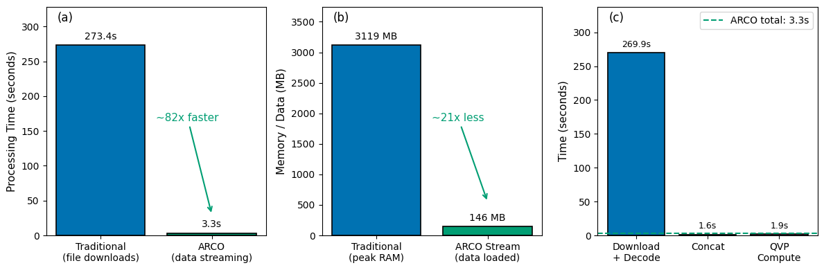
Key takeaway

ARCO’s advantage isn’t compression — it’s selective access. The traditional path downloads every sweep of every variable in every file (~809 MB compressed, ~3.2 GB decompressed) to extract the 146 MB it actually needs. ARCO streams exactly those 146 MB and nothing else. Once the data model and storage layer make that selectivity declarative — one .sel(vcp_time=slice(...)) instead of fifty lines of file iteration — the toil Abernathey et al. (2021) describe simply disappears.

The same pattern scales linearly with window length. Notebook 3 picks up here and pushes it from a single 4-hour window to seasonal QPE on a Dask cluster.

---

← Notebook 1 — NEXRAD KLOT Demo   ·   Notebook 3 — QPE Scaling Benchmark →

References

• Abernathey, R.P., T. Augspurger, A. Banihirwe, C.C. Blackmon-Luca, T.J. Crone, C.L. Gentemann, J.J. Hamman, N. Henderson, C. Lepore, T.A. McCaie, N.H. Robinson, and R.P. Signell, 2021: Cloud-Native Repositories for Big Scientific Data. Computing in Science & Engineering, 23, 26–35, https://doi.org/10.1109/MCSE.2021.3059437.

• Ryzhkov, A., P. Zhang, H. Reeves, M. Kumjian, T. Tschallener, S. Trömel, and C. Simmer, 2016: Quasi-Vertical Profiles—A New Way to Look at Polarimetric Radar Data. J. Atmos. Oceanic Technol., 33, 551–562, https://doi.org/10.1175/JTECH-D-15-0020.1.

• Wilkinson, M.D., et al., 2016: The FAIR Guiding Principles for scientific data management and stewardship. Scientific Data, 3, 160018, https://doi.org/10.1038/sdata.2016.18.

• Ladino-Rincón, A., et al. (2026). Radar DataTree: A FAIR and Cloud-Native Framework for Scalable Weather Radar Archives. (Manuscript in preparation.)

• Earlier preprint: arXiv:2510.24943, https://doi.org/10.48550/arXiv.2510.24943