Computing Snow Accumulation from the December 2025 Illinois Winter Storm

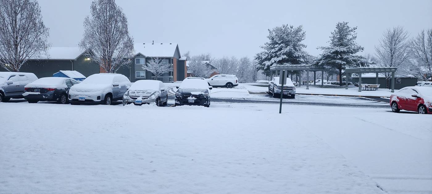
Computing Snow Accumulation from the December 2025 Illinois Winter Storm#

Snow-covered neighborhood in Illinois after a winter storm

Photo: A. Ladino-Rincon

The Storm: December 13-14, 2025#

A powerful winter storm moved through the Midwest, bringing heavy snowfall to northern Illinois. The NEXRAD radar at KLOT (Chicago) captured the entire event in real-time (see Notebook 1 for KLOT’s geographic coverage).

Storm Timeline:

December 13, 12:00 UTC: Snow begins spreading across northern Illinois
December 13, 18:00 UTC: Peak intensity, with heavy snowfall rates
December 14, 00:00 UTC: Snow continues, gradually tapering off
December 14, 06:00 UTC: Storm exits the region

import sys
import warnings
from pathlib import Path

warnings.filterwarnings("ignore", category=FutureWarning)

# Ensure demo_functions is importable (needed when executed from docs/)
sys.path.insert(0, str(Path("../notebooks").resolve()))

# Geographic visualization
import cartopy.crs as ccrs
import cartopy.feature as cfeature

# Radar-specific tools
import cmweather  # noqa: F401 - Radar colormaps
import icechunk as ic
import matplotlib.pyplot as plt
import numpy as np
import xarray as xr
from demo_functions import concat_sweep_across_vcps, rain_depth

print(f"xarray version: {xr.__version__}")
print(f"icechunk version: {ic.__version__}")

xarray version: 10000.dev6383+g8cf3ad708
icechunk version: 2.0.0a0

# Radar location (for reference in later calculations)
klot_lat = 41.6044
klot_lon = -88.0847

QPE Fundamentals: From Radar Reflectivity to Snow Depth#

The Challenge#

Weather radar measures reflectivity (Z), which tells us how much energy bounces back from precipitation particles. But what we want to know is how much snow fell - that requires converting Z into precipitation rate ®, then accumulating over time.

The Z-R Relationship#

The fundamental equation relating reflectivity to precipitation rate is:

\[Z = a \cdot R^b\]

Where:

Z: Radar reflectivity (in linear units, not dBZ)
R: Precipitation rate (mm/hr)
a, b: Empirical coefficients that depend on precipitation type

Rearranging to solve for R:

\[R = \left(\frac{Z}{a}\right)^{1/b}\]

Important

The key insight: Different precipitation types have different Z-R relationships because particle size, shape, and density vary.

Rain: Dense, uniform drops with predictable size distributions
Snow: Low-density aggregates with highly variable shapes

Rain vs Snow Coefficients#

Here are the empirical coefficients we’ll use:

Precipitation Type	a	b	Reference
Rain (Marshall-Palmer)	200	1.6	Marshall & Palmer (1948)
Snow (WSR-88D default)	75	2.0	Marshall-Gunn (1958)

Note

Why these coefficients? The WSR-88D (NEXRAD) operational snow algorithm uses a=75, b=2.0, which is based on Marshall & Gunn (1958). This relationship is well-validated for aggregate snow in the midlatitudes and gives reasonable accumulation estimates.

Tip

Z-S relationships vary widely! Values of ‘a’ range from 40 to 2000 in the literature. The WSR-88D default (a=75) is a good middle ground for typical winter storms. For specific storm types, different relationships may be more appropriate.

From Rates to Accumulation#

Once we have precipitation rate (mm/hr), we need to integrate over time to get total accumulation (mm):

\[\text{Accumulation} = \sum_{i=1}^{N} R_i \cdot \Delta t_i\]

Where:

\(R_i\): Precipitation rate at time step i
\(\Delta t_i\): Time interval between scans (typically 4-6 minutes for NEXRAD)

The rain_depth() function in demo_functions.py handles this automatically by:

Converting reflectivity from dBZ to linear units
Applying the Z-R relationship
Integrating over the vcp_time dimension

Note

Liquid equivalent vs actual snow depth

The output is in liquid equivalent (mm of water if the snow melted). To convert to actual snow depth, use the snow-to-liquid ratio (SLR):

\[\text{Snow Depth (inches)} = \text{Liquid Equivalent (inches)} \times \text{SLR}\]

Typical SLR values:

Wet, heavy snow: 5:1 to 10:1
Average: 10:1 to 15:1
Dry, fluffy snow: 15:1 to 30:1

We’ll use 10:1 (a conservative estimate) for this storm.

Accessing the Storm Data#

Now let’s connect to the KLOT radar archive and load the December 13-14 storm data.

Step 1: Connect to Icechunk Repository#

%%time
# Connect to KLOT data on Open Storage Network
storage = ic.s3_storage(
    bucket="nexrad-arco",
    prefix="KLOT-RT",
    endpoint_url="https://umn1.osn.mghpcc.org",
    anonymous=True,
    force_path_style=True,
    region="us-east-1",
)

# Open repository and create read-only session
repo = ic.Repository.open(storage)
session = repo.readonly_session("main")

print("Connected to KLOT radar archive")

Connected to KLOT radar archive
CPU times: user 42.8 ms, sys: 8.76 ms, total: 51.6 ms
Wall time: 359 ms

Step 2: Open DataTree#

%%time
# Open DataTree (lazy loading)
dtree = xr.open_datatree(
    session.store,
    zarr_format=3,
    consolidated=False,
    chunks={},
    engine="zarr",
    max_concurrency=5,
)

print(f"DataTree opened: {dtree.nbytes / 1024**3:.1f} GB total")
print(f"Available VCPs: {sorted(dtree.children)}")

# Show xarray's beautiful Dataset representation
dtree["VCP-34/sweep_0"].ds

DataTree opened: 94.2 GB total
Available VCPs: ['VCP-34']
CPU times: user 609 ms, sys: 119 ms, total: 728 ms
Wall time: 2.09 s

<xarray.DatasetView> Size: 17GB
Dimensions:            (vcp_time: 638, azimuth: 720, range: 1832)
Coordinates:
  * vcp_time           (vcp_time) datetime64[ns] 5kB 2025-12-08T21:04:51 ... ...
  * azimuth            (azimuth) float64 6kB 0.25 0.75 1.25 ... 359.2 359.8
    elevation          (azimuth) float64 6kB dask.array<chunksize=(720,), meta=np.ndarray>
    time               (azimuth) datetime64[ns] 6kB dask.array<chunksize=(720,), meta=np.ndarray>
  * range              (range) float32 7kB 2.125e+03 2.375e+03 ... 4.599e+05
    x                  (azimuth, range) float64 11MB dask.array<chunksize=(180, 458), meta=np.ndarray>
    z                  (azimuth, range) float64 11MB dask.array<chunksize=(180, 458), meta=np.ndarray>
    y                  (azimuth, range) float64 11MB dask.array<chunksize=(180, 458), meta=np.ndarray>
    altitude           int64 8B ...
    crs_wkt            int64 8B ...
    latitude           float64 8B ...
    longitude          float64 8B ...
Data variables:
    CCORH              (vcp_time, azimuth, range) float32 3GB dask.array<chunksize=(1, 720, 1832), meta=np.ndarray>
    DBZH               (vcp_time, azimuth, range) float32 3GB dask.array<chunksize=(1, 720, 1832), meta=np.ndarray>
    ZDR                (vcp_time, azimuth, range) float32 3GB dask.array<chunksize=(1, 720, 1832), meta=np.ndarray>
    PHIDP              (vcp_time, azimuth, range) float32 3GB dask.array<chunksize=(1, 720, 1832), meta=np.ndarray>
    RHOHV              (vcp_time, azimuth, range) float32 3GB dask.array<chunksize=(1, 720, 1832), meta=np.ndarray>
    sweep_fixed_angle  (vcp_time) float32 3kB dask.array<chunksize=(1,), meta=np.ndarray>
    sweep_number       (vcp_time) float64 5kB dask.array<chunksize=(1,), meta=np.ndarray>

Handling Multi-VCP Data: The Continuous Storm Challenge#

The Problem#

During a storm, the radar automatically switches between different Volume Coverage Patterns (VCPs) based on weather conditions:

Timeline:
├─ 12:00 UTC: VCP-34 (clear air mode)
├─ 14:00 UTC: VCP-212 (precipitation mode) ← Radar detects intensifying storm
├─ 18:00 UTC: VCP-35 (severe weather mode) ← Peak intensity
└─ 22:00 UTC: VCP-212 (precipitation mode) ← Storm weakens

Each VCP has its own hierarchical branch in the DataTree. If we only load one VCP, we’d have gaps in our time series.

Warning

Common mistake: Computing accumulation from a single VCP will underestimate total snowfall because you’re missing entire time periods when other VCPs were active.

The Solution: Concatenate Across VCPs#

The concat_sweep_across_vcps() function (from demo_functions.py) solves this by:

Finding all VCP nodes in the DataTree
Extracting the same sweep (e.g., sweep_0) from each VCP
Concatenating them along the vcp_time dimension
Sorting by time to create a continuous time series

# Example usage
continuous_data = concat_sweep_across_vcps(
    dtree,
    sweep_name="sweep_0",  # Lowest elevation angle
    append_dim="vcp_time",
    sort_by_time=True       # Ensure chronological order
)

Tip

Why sweep_0?

For QPE (precipitation accumulation), we use the lowest elevation sweep (sweep_0) because:

It’s closest to the ground (where we want to measure accumulation)
All VCPs include sweep_0, ensuring compatibility
Higher sweeps sample the atmosphere aloft, not surface precipitation

Step 3: Create Continuous Time Series#

Let’s concatenate sweep_0 across all VCPs to create an uninterrupted storm record:

%%time
# Concatenate sweep_0 across all VCPs
sweep_0_continuous = concat_sweep_across_vcps(
    dtree,
    sweep_name="sweep_0",
    append_dim="vcp_time",
    validate_coords=True,  # Verify spatial compatibility
    sort_by_time=True,  # Chronological order
)

print("Continuous dataset created")
print(
    f"Time span: {sweep_0_continuous.vcp_time.min().values} to {sweep_0_continuous.vcp_time.max().values}"
)
print(f"Number of scans: {len(sweep_0_continuous.vcp_time)}")
print(f"Variables: {list(sweep_0_continuous.data_vars)}")

Continuous dataset created
Time span: 2025-12-08T21:04:51.000000000 to 2025-12-14T01:15:42.000000000
Number of scans: 638
Variables: ['CCORH', 'DBZH', 'ZDR', 'PHIDP', 'RHOHV', 'sweep_fixed_angle', 'sweep_number']
CPU times: user 12.9 ms, sys: 1.11 ms, total: 14 ms
Wall time: 13.6 ms

Step 4: Select Storm Time Window#

Now we can directly slice the time period of interest:

# Define storm period (December 13, 12:00 UTC to December 14, 06:00 UTC)
STORM_START = "2025-12-13T12:00"
STORM_END = "2025-12-14T06:00"

# Select storm window
storm_data = sweep_0_continuous.sel(vcp_time=slice(STORM_START, STORM_END))

num_scans = len(storm_data.vcp_time)
duration_hours = (
    (storm_data.vcp_time[-1] - storm_data.vcp_time[0])
    .values.astype("timedelta64[h]")
    .astype(int)
)

print("Storm window selected:")
print(f"  Start: {storm_data.vcp_time.min().values}")
print(f"  End: {storm_data.vcp_time.max().values}")
print(f"  Duration: {duration_hours} hours")
print(f"  Number of scans: {num_scans}")
print(f"  Average scan interval: {duration_hours * 60 / num_scans:.1f} minutes")

Storm window selected:
  Start: 2025-12-13T12:09:20.000000000
  End: 2025-12-14T01:15:42.000000000
  Duration: 13 hours
  Number of scans: 85
  Average scan interval: 9.2 minutes

Visualizing Storm Evolution#

Before computing accumulation, let’s see how reflectivity evolved during the storm:

# Sample 6 evenly-spaced time points throughout the storm
sample_indices = np.linspace(0, len(storm_data.vcp_time) - 1, 6, dtype=int)

fig, axes = plt.subplots(2, 3, figsize=(12, 8))
axes = axes.flatten()

for idx, time_idx in enumerate(sample_indices):
    scan = storm_data.isel(vcp_time=time_idx)
    time_str = str(scan.vcp_time.values)[:16].replace("T", " ")

    scan.DBZH.plot(
        ax=axes[idx],
        x="x",
        y="y",
        cmap="ChaseSpectral",
        vmin=-10,
        vmax=50,
        add_colorbar=True,
        cbar_kwargs={"label": "dBZ", "shrink": 0.8},
    )
    axes[idx].set_title(f"{time_str} UTC", fontsize=10, fontweight="bold")
    axes[idx].set_xlabel("East (m)", fontsize=9)
    axes[idx].set_ylabel("North (m)", fontsize=9)
    axes[idx].set_aspect("equal")

fig.suptitle(
    "December 2025 Winter Storm - Reflectivity Evolution",
    fontsize=12,
    fontweight="bold",
    y=0.995,
)
plt.tight_layout(rect=[0, 0, 1, 0.99])
plt.show()

print(f"✓ Displayed storm evolution across {len(sample_indices)} time steps")

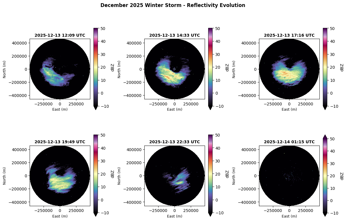
_images/fcbe4a7b21b3958f190db21625a7a83f04ad1793dfaa55e24dda7546df9b55a5.png

✓ Displayed storm evolution across 6 time steps

Computing Snow Accumulation#

Now comes the main event: converting reflectivity into snowfall accumulation.

The Process#

We’ll use the rain_depth() function with WSR-88D snow coefficients:

a = 75 (Marshall-Gunn)
b = 2.0

The function will:

Convert DBZH from dBZ to linear units
Apply the Z-S relationship: \(R = (Z/75)^{1/2.0}\)
Integrate precipitation rates over the vcp_time dimension
Return total liquid equivalent accumulation (mm)

Note

This computation happens lazily - the data only streams when we call .compute().

%%time
# Compute snow accumulation (liquid equivalent)
# Using WSR-88D snow coefficients (Marshall-Gunn 1958)
snow_depth_per_scan = rain_depth(
    storm_data.DBZH,
    a=75,  # WSR-88D snow coefficient
    b=2.0,  # WSR-88D snow coefficient
    t=None,  # Auto-compute from vcp_time dimension
)

# Sum over time to get total accumulation and load into memory
snow_accumulation = snow_depth_per_scan.sum(dim="vcp_time", skipna=True).compute()

print("\nSnow accumulation computed successfully")
print(f"Result shape: {snow_accumulation.shape}")
print(f"Dimensions: {snow_accumulation.dims}")

Actual QPE integration period: 0 days, 13 hours, 6 minutes
Time span: 2025-12-13T12:09:20 to 2025-12-14T01:15:42 UTC

Snow accumulation computed successfully
Result shape: (720, 1832)
Dimensions: ('azimuth', 'range')
CPU times: user 2.94 s, sys: 308 ms, total: 3.25 s
Wall time: 2.11 s

Geographic Visualization: Where Did the Snow Fall?#

Now let’s create a map showing snow accumulation across northern Illinois.

# Convert accumulation to inches for U.S. audience
snow_accumulation_inches = snow_accumulation * (1 / 25.4)

# Estimate snow depth (using 10:1 SLR)
snow_depth_inches = snow_accumulation_inches * 10

# KLOT radar location
klot_lat = 41.6044
klot_lon = -88.0847

# Create geographic map with cartopy
fig = plt.figure(figsize=(10, 8))
ax = plt.axes(
    projection=ccrs.LambertConformal(
        central_longitude=klot_lon, central_latitude=klot_lat
    )
)

# Set extent to cover radar domain (~250 km around radar)
ax.set_extent(
    [klot_lon - 3.5, klot_lon + 3.5, klot_lat - 2.5, klot_lat + 2.5],
    crs=ccrs.PlateCarree(),
)

# Add geographic features
ax.add_feature(cfeature.STATES, linewidth=1.5, edgecolor="black", zorder=3)
ax.add_feature(cfeature.COASTLINE, linewidth=1, zorder=3)
ax.add_feature(cfeature.LAKES, alpha=0.5, facecolor="lightblue", zorder=2)

# Plot snow accumulation using x/y coordinates (meters from radar)
# Transform x/y from radar-centered meters to lat/lon for plotting
if "x" in snow_depth_inches.coords and "y" in snow_depth_inches.coords:
    # Get x, y coordinates (in meters from radar)
    x_vals = snow_depth_inches.x.values  # 2D array
    y_vals = snow_depth_inches.y.values  # 2D array

    # Convert to approximate lat/lon (simple offset from radar location)
    # Note: This is approximate; for exact georeferencing use pyproj
    lon_vals = klot_lon + (x_vals / 111000) / np.cos(np.radians(klot_lat))
    lat_vals = klot_lat + (y_vals / 111000)

    # Plot with pcolormesh for geographic overlay
    p2, p98 = np.nanpercentile(snow_depth_inches.values, [2, 98])
    im = ax.pcolormesh(
        lon_vals,
        lat_vals,
        snow_depth_inches.values,
        cmap="Blues",
        vmin=0,
        vmax=max(p98, 1),
        transform=ccrs.PlateCarree(),
        zorder=1,
        alpha=0.8,
    )
    plt.colorbar(im, ax=ax, label="Est. Snow Depth (in)", shrink=0.7, pad=0.02)

# Mark radar location
ax.plot(
    klot_lon,
    klot_lat,
    marker="*",
    markersize=20,
    color="red",
    markeredgecolor="black",
    markeredgewidth=1.5,
    transform=ccrs.PlateCarree(),
    label="KLOT Radar",
    zorder=10,
)

# Add city markers
cities = {
    "Chicago": (41.8781, -87.6298),
    "Rockford": (42.2711, -89.0940),
    "Joliet": (41.5250, -88.0817),
}
for city, (lat, lon) in cities.items():
    ax.plot(
        lon,
        lat,
        marker="o",
        markersize=6,
        color="black",
        transform=ccrs.PlateCarree(),
        zorder=9,
    )
    ax.text(
        lon + 0.12,
        lat,
        city,
        fontsize=9,
        transform=ccrs.PlateCarree(),
        ha="left",
        fontweight="bold",
        bbox=dict(facecolor="white", alpha=0.7, edgecolor="none", pad=1),
    )

ax.gridlines(draw_labels=True, dms=True, x_inline=False, y_inline=False, alpha=0.3)
ax.legend(loc="upper right", fontsize=10)
ax.set_title(
    "December 13-14, 2025 Snow Accumulation\nNEXRAD KLOT (10:1 SLR)",
    fontsize=12,
    fontweight="bold",
)

plt.tight_layout()
plt.savefig(
    "snow_accumulation_map.png", dpi=150, bbox_inches="tight", facecolor="white"
)
plt.show()

print(f"\n✓ Figure saved. Color scale: 0 to {max(p98, 1):.1f} inches (98th percentile)")

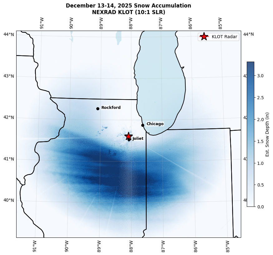
_images/aba47191108dc1fc71cf0cc30394b210feab356114239a112f03a170a3b74c19.png

✓ Figure saved. Color scale: 0 to 3.3 inches (98th percentile)

Cross-Sections: Accumulation Profiles#

Let’s examine accumulation along transects through the domain:

fig, (ax1, ax2) = plt.subplots(1, 2, figsize=(12, 4))

# Radial profile (average across all azimuths)
range_km = snow_depth_inches.range.values / 1000
radial_profile = snow_depth_inches.mean(dim="azimuth", skipna=True)

ax1.plot(range_km, radial_profile.values, "b-", linewidth=2)
ax1.axvline(0, color="red", linestyle="--", linewidth=1.5, label="Radar", alpha=0.7)
ax1.set_xlabel("Distance from Radar (km)", fontsize=10)
ax1.set_ylabel("Est. Snow Depth (in)", fontsize=10)
ax1.set_title("Radial Profile (Azimuth Average)", fontsize=11, fontweight="bold")
ax1.legend(fontsize=9)
ax1.grid(alpha=0.3)
ax1.set_xlim(0, 230)
# Auto-scale y-axis based on data
ax1.set_ylim(0, max(radial_profile.max().values * 1.1, 0.5))

# Azimuthal profile at 100 km range
target_range_m = 100000
az_profile = snow_depth_inches.sel(range=target_range_m, method="nearest")

ax2.plot(az_profile.azimuth.values, az_profile.values, "g-", linewidth=2)
ax2.set_xlabel("Azimuth (degrees)", fontsize=10)
ax2.set_ylabel("Est. Snow Depth (in)", fontsize=10)
ax2.set_title("Azimuthal Profile at 100 km", fontsize=11, fontweight="bold")
ax2.grid(alpha=0.3)
ax2.set_xlim(0, 360)
# Auto-scale y-axis
ax2.set_ylim(0, max(float(az_profile.max(skipna=True).values) * 1.1, 0.5))
for az, label in [(0, "N"), (90, "E"), (180, "S"), (270, "W")]:
    ax2.axvline(az, color="gray", linestyle=":", alpha=0.5)
    ax2.text(az, ax2.get_ylim()[1] * 0.9, label, ha="center", fontsize=9)

plt.tight_layout()
plt.show()

print(f"Max radial accumulation: {radial_profile.max().values:.2f} inches")
print(
    f"Max azimuthal accumulation at 100 km: {az_profile.max(skipna=True).values:.2f} inches"
)

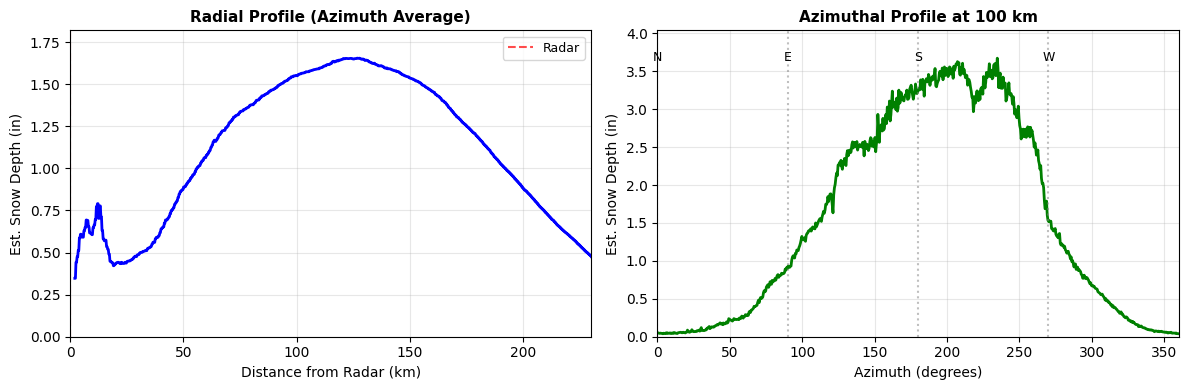
_images/85f9b0694b13b14b7bac973338e7c1a59355bccbda4fa15f56c58bc82ba3f05e.png

Max radial accumulation: 1.65 inches
Max azimuthal accumulation at 100 km: 3.67 inches

Scientific Integrity: Understanding Your Results#

Every radar-derived estimate has inherent uncertainty. Knowing these limits is what separates credible analysis from naive code execution.

Key Sources of Uncertainty#

Source	Impact	Notes
Z-R coefficients	±30–70%	Snowflake density, size, and crystal habit vary with temperature and humidity
Beam height	Increases with range	At far ranges the beam samples well above the surface; estimates most reliable within ~100 km
Bright band	Overestimation	Melting snow produces artificially high reflectivity; QVPs help identify this
Ground clutter / blockage	Localized errors	Buildings, terrain can block or reflect the beam
SLR assumption	±50%+	We used 10:1, but real SLR ranges from 5:1 (wet snow) to 30:1+ (dry, fluffy snow)

Tip

For publications, include a statement like: “Radar-derived QPE estimates have typical uncertainties of ±30–50% for snow events (Roebber et al., 2003). Validation against surface observations is recommended.”

Validation Strategy (Future Work)#

To improve confidence in radar QPE:

Ground truth comparison:
- CoCoRaHS volunteer observations
- Automated ASOS/AWOS stations
- Snowboard measurements
Multi-sensor fusion:
- Combine radar with satellite (MRMS products)
- Gauge correction factors
- Model QPF for storm structure
Improved Z-S relationships:
- Use polarimetric variables (ZDR, KDP) to classify snow type
- Apply different coefficients for different hydrometeor classes
- Adjust for temperature profiles

Tip

Research opportunity: Compare your radar estimates with official snowfall reports. Where do they agree? Disagree? Why might that be?

Summary: What You’ve Accomplished#

You just computed snowfall accumulation for an entire winter storm — from your laptop!

This is publication-quality analysis. Seriously. You now have the skills to analyze any winter storm in the 30+ year NEXRAD archive.

Skills You’ve Mastered#

QPE fundamentals:
- Z-R relationships for rain vs snow
- Time integration to compute accumulation
- Liquid equivalent vs actual snow depth
Multi-VCP data handling:
- Used concat_sweep_across_vcps() for continuous time series
- Understood why radar switches VCPs during storms
Cloud-native workflows:
- Connected to KLOT archive on OSN
- Streamed only the data needed (sweep_0, storm window)
- Computed accumulation without downloading files
Scientific visualization:
- Geographic accumulation maps
- Storm evolution time series
- Radial and azimuthal profiles
Scientific integrity:
- Z-R relationship variability
- Beam height effects
- Uncertainty quantification and communication

The Big Picture#

This workflow would have been:

Impossible 10 years ago (data not archived at this resolution)
Tedious 5 years ago (download hundreds of files, decode each one)
Trivial today (stream on-demand, compute in memory)

This is the power of FAIR, cloud-native data.

Next Steps: Extend Your Analysis#

Challenge Yourself

Ready to go deeper? Try these extensions:

Compare with ground truth: Download snowfall reports from CoCoRaHS and compare with radar estimates
Improve the Z-S relationship: Use ZDR and KDP for hydrometeor classification
Analyze storm structure: Compute QVPs to see vertical structure
Scale to other storms: Analyze the entire winter season (December-February)

References#

Z-R Relationships#

Marshall, J. S., & Palmer, W. M. (1948). The distribution of raindrops with size. Journal of Meteorology, 5(4), 165-166.
Marshall, J. S., & Gunn, K. L. S. (1958). Measurement of snow parameters by radar. Journal of Meteorology, 15(2), 209-215. (Used for WSR-88D snow algorithm)

Radar QPE Techniques#

Cifelli, R., Chandrasekar, V., Lim, S., Kennedy, P. C., Wang, Y., & Rutledge, S. A. (2011). A new dual-polarization radar rainfall algorithm: Application in Colorado precipitation events. Journal of Atmospheric and Oceanic Technology, 28(3), 352-364.
Gourley, J. J., et al. (2017). The FLASH Project: Improving the Tools for Flash Flood Monitoring and Prediction across the United States. Bulletin of the American Meteorological Society, 98(2), 361-372.

Snow-to-Liquid Ratios#

Roebber, P. J., Bruening, S. L., Schultz, D. M., & Cortinas Jr, J. V. (2003). Improving snowfall forecasting by diagnosing snow density. Weather and Forecasting, 18(2), 264-287.

Radar DataTree Framework#

Ladino-Rincón, A., & Nesbitt, S. W. (2025). Radar DataTree: A FAIR and Cloud-Native Framework for Scalable Weather Radar Archives. arXiv preprint arXiv:2510.24943. https://doi.org/10.48550/arXiv.2510.24943

Citation#

If you use this notebook or framework in your research, please cite:

Ladino-Rincón, A., & Nesbitt, S. W. (2025). Radar DataTree: A FAIR and Cloud-Native Framework for Scalable Weather Radar Archives. arXiv:2510.24943. doi:10.48550/arXiv.2510.24943

Tutorial created by the Radar DataTree team

Last updated: February 2025

Computing Snow Accumulation from the December 2025 Illinois Winter Storm

Contents

Computing Snow Accumulation from the December 2025 Illinois Winter Storm#

The Storm: December 13-14, 2025#

QPE Fundamentals: From Radar Reflectivity to Snow Depth#

The Challenge#

The Z-R Relationship#

Rain vs Snow Coefficients#

From Rates to Accumulation#

Accessing the Storm Data#

Step 1: Connect to Icechunk Repository#

Step 2: Open DataTree#

Handling Multi-VCP Data: The Continuous Storm Challenge#

The Problem#

The Solution: Concatenate Across VCPs#

Step 3: Create Continuous Time Series#

Step 4: Select Storm Time Window#

Visualizing Storm Evolution#

Computing Snow Accumulation#

The Process#

Geographic Visualization: Where Did the Snow Fall?#

Cross-Sections: Accumulation Profiles#

Scientific Integrity: Understanding Your Results#

Key Sources of Uncertainty#

Validation Strategy (Future Work)#

Summary: What You’ve Accomplished#

Skills You’ve Mastered#

The Big Picture#

Next Steps: Extend Your Analysis#

Related Notebooks#

References#

Z-R Relationships#

Radar QPE Techniques#

Snow-to-Liquid Ratios#

Radar DataTree Framework#

Citation#