



Get only the sweep you need#
Most analyses only ever want the bottom of the volume: the cuts closest to the ground, where the precipitation actually is. On a WSR-88D that is sweep_0 and sweep_1 — and in the native archive they are scattered across every Volume Coverage Pattern the radar has ever run, each with its own timeline.
KLOT-lowsweeps publishes exactly those two sweeps as one flat, time-sorted dataset. Building it copied no data: its chunks are byte-range references into the ARCO chunks already stored in s3://nexrad-arco/. It is a second, purpose-shaped view over one physical copy — not a second copy of it. This notebook opens it, explains why there are two sweeps at the same elevation, and plots the polarimetric view.
TL;DR
If you only need the lowest cuts, open KLOT-lowsweeps and skip the VCP bookkeeping entirely — sweep_0 and sweep_1 arrive as single continuous time axes spanning the whole archive. We show why those two sweeps sit at the same elevation angle, then plot Z, ZDR, RHOHV and PHIDP for a March 2026 severe storm over Chicago.
Prerequisites
This notebook builds on Notebook 1 — NEXRAD KLOT Demo:
connecting to the public archive with an anonymous Icechunk session
opening a DataTree with
engine="rustytree"selecting a scan with
.sel(vcp_time=..., method="nearest")and georeferencing it
Notebook 1 plots reflectivity for a single scan pulled from one VCP. Here we take the low sweep as one continuous series spanning the whole archive, and all four polarimetric moments.
Why the low sweeps need their own dataset#
A NEXRAD radar switches Volume Coverage Patterns as the weather changes — rapid-scan VCP-212 in severe convection, VCP-31 in clear air, and so on. Each VCP is a separate node in the native DataTree with its own vcp_time axis, and each carries its own low sweeps. Reaching “the lowest cut, over years” therefore means walking every VCP node and stitching their timelines together — every time, for every analysis.
That assembly is identical for everyone, so it has been done once, and the result is shaped like the question people actually ask.
Virtual references — reshape without copying
KLOT-lowsweeps stores almost no data of its own. Its chunks are byte-range references into objects already sitting in s3://nexrad-arco/, so the archive is re-indexed rather than duplicated. That is what makes a purpose-shaped dataset cheap to publish: many convenient views, one physical copy.
Tools like VirtualiZarr build these reference sets; here they are produced by the raw2zarr pipeline. Reading one requires authorizing the container the references point into — see the next section.
import icechunk as ic
import xarray as xr
import xradar  # noqa: F401  — registers the .xradar accessor
Open the virtual archive#
Same idea as Notebook 1, with one addition: this repo’s chunks are references into s3://nexrad-arco/, so reading its data means authorizing that container. In Arraylake that is a bucket nickname:
from arraylake import Client  # pip install arraylake

repo = Client().get_repo(
    "atmoscale/KLOT-lowsweeps",
    authorize_virtual_chunk_access={"s3://nexrad-arco/": "nexrad-arco"},
)
session = repo.readonly_session("main")
As in Notebook 1, that needs an Arraylake account and access to the atmoscale organization. The cell below is the credential-free icechunk equivalent — expand it for the anonymous form.
<xarray.DataTree>
Group: /
│   Dimensions:      ()
│   Coordinates:
│       follow_mode  object 8B ...
│       prt_mode     object 8B ...
│       sweep_mode   object 8B ...
├── Group: /sweep_0
│       Dimensions:              (vcp_time: 1018162, azimuth: 720, range: 1832)
│       Coordinates:
│         * vcp_time             (vcp_time) datetime64[ns] 8MB 2015-01-01T00:09:35.13...
│         * azimuth              (azimuth) float64 6kB 0.25 0.75 1.25 ... 359.2 359.8
│           elevation            (azimuth) float64 6kB dask.array<chunksize=(720,), meta=np.ndarray>
│           time                 (vcp_time, azimuth) datetime64[ns] 6GB dask.array<chunksize=(1, 720), meta=np.ndarray>
│         * range                (range) float32 7kB 2.125e+03 2.375e+03 ... 4.599e+05
│           altitude             float64 8B ...
│           latitude             float64 8B ...
│           longitude            float64 8B ...
│       Data variables:
│           DBZH                 (vcp_time, azimuth, range) float32 5TB dask.array<chunksize=(1, 720, 1832), meta=np.ndarray>
│           PHIDP                (vcp_time, azimuth, range) float32 5TB dask.array<chunksize=(1, 720, 1832), meta=np.ndarray>
│           RHOHV                (vcp_time, azimuth, range) float32 5TB dask.array<chunksize=(1, 720, 1832), meta=np.ndarray>
│           ZDR                  (vcp_time, azimuth, range) float32 5TB dask.array<chunksize=(1, 720, 1832), meta=np.ndarray>
│           ray_elevation_angle  (vcp_time, azimuth) float64 6GB dask.array<chunksize=(1, 720), meta=np.ndarray>
│           sweep_fixed_angle    (vcp_time) float32 4MB dask.array<chunksize=(1,), meta=np.ndarray>
│           sweep_number         (vcp_time) float32 4MB dask.array<chunksize=(1,), meta=np.ndarray>
│       Attributes:
│           base_tilt_cut:          False
│           channel_config:         sz2_phase_coding
│           mpda_cut:               False
│           mrle_cut:               False
│           mrle_sequence_number:   0
│           sails_cut:              False
│           sails_sequence_number:  0
│           super_resolution:       11
│           waveform_type:          contiguous_surveillance
└── Group: /sweep_1
        Dimensions:              (vcp_time: 1018162, azimuth: 720, range: 1192)
        Coordinates:
          * vcp_time             (vcp_time) datetime64[ns] 8MB 2015-01-01T00:09:35.13...
          * azimuth              (azimuth) float64 6kB 0.25 0.75 1.25 ... 359.2 359.8
            elevation            (azimuth) float64 6kB dask.array<chunksize=(720,), meta=np.ndarray>
            time                 (vcp_time, azimuth) datetime64[ns] 6GB dask.array<chunksize=(1, 720), meta=np.ndarray>
          * range                (range) float32 5kB 2.125e+03 2.375e+03 ... 2.999e+05
            altitude             float64 8B ...
            latitude             float64 8B ...
            longitude            float64 8B ...
        Data variables:
            DBZH                 (vcp_time, azimuth, range) float32 3TB dask.array<chunksize=(1, 720, 1192), meta=np.ndarray>
            VRADH                (vcp_time, azimuth, range) float32 3TB dask.array<chunksize=(1, 720, 1192), meta=np.ndarray>
            WRADH                (vcp_time, azimuth, range) float32 3TB dask.array<chunksize=(1, 720, 1192), meta=np.ndarray>
            ray_elevation_angle  (vcp_time, azimuth) float64 6GB dask.array<chunksize=(1, 720), meta=np.ndarray>
            sweep_fixed_angle    (vcp_time) float32 4MB dask.array<chunksize=(1,), meta=np.ndarray>
            sweep_number         (vcp_time) float32 4MB dask.array<chunksize=(1,), meta=np.ndarray>
        Attributes:
            base_tilt_cut:          False
            channel_config:         sz2_phase_coding
            mpda_cut:               False
            mrle_cut:               False
            mrle_sequence_number:   0
            sails_cut:              False
            sails_sequence_number:  0
            super_resolution:       7
waveform_type: contiguous_doppler# A flat tree: two sweeps, each already one continuous series.
ds_low = dt_low["sweep_0"].to_dataset(inherit="all_coords")
ds_doppler = dt_low["sweep_1"].to_dataset(inherit="all_coords")
print(
f"sweep_0: {ds_low.sizes['vcp_time']:,} scans "
f"({str(ds_low.vcp_time.values.min())[:10]} -> {str(ds_low.vcp_time.values.max())[:10]})"
)
print(f"sweep_1: {ds_doppler.sizes['vcp_time']:,} scans")
# Proof that this dataset is a re-indexing, not a copy: ask the store what kind
# of chunk backs a variable and it reports a reference to another object.
print(f"chunk type of sweep_0/DBZH: {session.chunk_type('/sweep_0/DBZH', (0, 0, 0))}")
sweep_0: 1,018,162 scans (2015-01-01 -> 2026-10-06)
sweep_1: 1,018,162 scans
chunk type of sweep_0/DBZH: ChunkType.virtual
Two sweeps, one elevation: the split cut#
sweep_0 and sweep_1 are not two different heights. They are the same 0.5° tilt scanned twice, because no single pulse scheme measures reflectivity and velocity well at once:
a long pulse interval sees far without range ambiguity, but folds velocity;
a short pulse interval measures velocity cleanly, but wraps distant echoes.
So the radar does both and reports them as consecutive sweeps — the split cut. Ask the data rather than taking that on trust:
import pandas as pd

MOMENTS = ("DBZH", "ZDR", "RHOHV", "PHIDP", "VRADH", "WRADH")
split_cut = pd.DataFrame(
    {
        name: {
            "elevation [deg]": round(
                float(ds.sweep_fixed_angle.isel(vcp_time=0).compute()), 2
            ),
            "gates": ds.sizes["range"],
            "max range [km]": round(float(ds.range.max()) / 1000),
            "moments": ", ".join(m for m in MOMENTS if m in ds.data_vars),
        }
        for name, ds in [("sweep_0", ds_low), ("sweep_1", ds_doppler)]
    }
).T
split_cut
| elevation [deg] | gates | max range [km] | moments | |
|---|---|---|---|---|
| sweep_0 | 0.48 | 1832 | 460 | DBZH, ZDR, RHOHV, PHIDP |
| sweep_1 | 0.48 | 1192 | 300 | DBZH, VRADH, WRADH |
Same angle, different jobs. sweep_0 is the surveillance cut — it reaches 460 km and carries the polarimetric moments (ZDR, RHOHV, PHIDP) that describe what the hydrometeors are. sweep_1 is the Doppler cut — shorter reach, but it carries VRADH and WRADH, which describe how they move.
Reach for sweep_0 for precipitation type and rainfall estimation; reach for sweep_1 for rotation and wind. Both are one .sel() away below.
Pull one scan#
Selecting a moment is a single .sel() — now spanning the entire archive rather than one VCP.
# A severe storm over Chicago on the evening of 10 March 2026.
scan = ds_low.sel(vcp_time="2026-03-10 23:10", method="nearest").xradar.georeference()
scan
<xarray.Dataset> Size: 53MB
Dimensions:              (azimuth: 720, range: 1832)
Coordinates: (12/15)
  * azimuth              (azimuth) float64 6kB 0.25 0.75 1.25 ... 359.2 359.8
    elevation            (azimuth) float64 6kB dask.array<chunksize=(720,), meta=np.ndarray>
    time                 (azimuth) datetime64[ns] 6kB dask.array<chunksize=(720,), meta=np.ndarray>
  * range                (range) float32 7kB 2.125e+03 2.375e+03 ... 4.599e+05
    x                    (azimuth, range) float64 11MB dask.array<chunksize=(720, 1832), meta=np.ndarray>
    y                    (azimuth, range) float64 11MB dask.array<chunksize=(720, 1832), meta=np.ndarray>
    ...                   ...
    sweep_mode           object 8B ...
    altitude             float64 8B ...
    latitude             float64 8B ...
    longitude            float64 8B ...
    vcp_time             datetime64[ns] 8B 2026-03-10T23:08:53.341000080
    crs_wkt              int64 8B 0
Data variables:
    DBZH                 (azimuth, range) float32 5MB dask.array<chunksize=(720, 1832), meta=np.ndarray>
    PHIDP                (azimuth, range) float32 5MB dask.array<chunksize=(720, 1832), meta=np.ndarray>
    RHOHV                (azimuth, range) float32 5MB dask.array<chunksize=(720, 1832), meta=np.ndarray>
    ZDR                  (azimuth, range) float32 5MB dask.array<chunksize=(720, 1832), meta=np.ndarray>
    ray_elevation_angle  (azimuth) float64 6kB dask.array<chunksize=(720,), meta=np.ndarray>
    sweep_fixed_angle    float32 4B dask.array<chunksize=(), meta=np.ndarray>
    sweep_number         float32 4B dask.array<chunksize=(), meta=np.ndarray>
Attributes:
    base_tilt_cut:          False
    channel_config:         sz2_phase_coding
    mpda_cut:               False
    mrle_cut:               False
    mrle_sequence_number:   0
    sails_cut:              False
    sails_sequence_number:  0
    super_resolution:       11
waveform_type: contiguous_surveillanceplot_polarimetric_panel(scan)
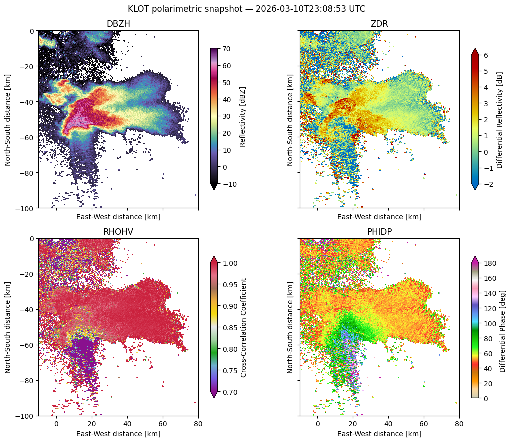
What the four moments tell you. This is why it is worth carrying the polarimetric variables rather than reflectivity alone.
Z alone shows an intense core — around 44 dBZ typical, 60 dBZ at peak.
ZDR is strongly positive (+2 dB, locally 4–6 dB) through that core: the scatterers are wide and flattened, i.e. large oblate raindrops and melting hydrometeors.
RHOHV stays near 0.98 across the precipitation, confirming a uniform population of meteorological targets.
PHIDP accumulates steadily outward along each radial, the propagation signature of rain-path liquid water.
Then there is the narrow plume extending away from the radar just beyond the core, where RHOHV collapses to ~0.66 and ZDR goes slightly negative. It is tempting to read any low-RHOHV plume as tornadic debris, but the reflectivity there is only ~2 dBZ — debris is a strong scatterer, so a debris signature comes with high Z. Weak echo, decorrelated, directly behind a hail-bearing core is instead a three-body scatter spike: energy bounces hail → ground → hail → radar, arriving late and so plotted too far out. It is an artifact, not weather — and one that reflectivity alone would not let you identify.
Confirming rotation would need the velocity field, which lives in sweep_1 — the Doppler half of the split cut.
Where to next#
One call, one time axis, one scan — because the dataset was shaped around the question. The analysis notebooks take it from here:
Reproduce a published figure? → Notebook 3 — QVP comparison reproduces Ryzhkov et al. (2016) Fig. 4 and benchmarks ARCO streaming against the traditional file workflow.
Estimate rainfall accumulation? → Notebook 4 — QPE scaling applies the Marshall–Palmer Z–R relation to exactly this low sweep, live for one day and scaling to seasons on a cluster.
← Notebook 1 — NEXRAD KLOT Demo
Cite this work: Ladino-Rincón, A., et al. (2026). Radar DataTree: A Cloud-Native AI-Ready Data Model for Accessible, Time-Aware Weather Radar Datasets. Submitted to IEEE Transactions on Big Data. Earlier preprint: arXiv:2510.24943, doi:10.48550/arXiv.2510.24943.