QPE Scaling Benchmark: From Hours to Months

QPE Scaling Benchmark: From Hours to Months#

This notebook is the QPE companion to Ladino-Rincón et al. (2026, submitted to IEEE Transactions on Big Data). It computes a Quantitative Precipitation Estimate (QPE) accumulation over the 24-hour KVNX MCS event using the same ARCO streaming pattern as Notebook 3, then sketches the path for scaling the same code to weeks, months, or seasons on a cluster.

The scientific product here is rainfall depth from the lowest-elevation sweep (sweep_0 ≈ 0.5°), accumulated through time using the Marshall–Palmer Z–R relationship. The infrastructure story: one declarative selection delivers a 1-day, 1-week, or 6-month accumulation — only the time slice changes, and only the bytes you slice are streamed.

TL;DR

Compute Marshall–Palmer rainfall accumulation for a full day in seconds — and scale the same code to 7 days, 30 days, or a 6-month season on a Dask cluster using the recipes below. The paper reports speedups of 112× to 1,565× over the file-based path; ARCO streaming is what makes seasonal-scale radar QPE feasible without downloading terabytes.

Prerequisites

This notebook builds on the patterns introduced in:

Notebook 1 — anonymous icechunk session, engine="rustytree", glob-pattern open
Notebook 3 — time-window selection, ARCO chunk streaming, vcp_time.sel() slicing

What is a QPE?#

This notebook applies QPE to the May 20, 2011 KVNX MCS event from the MC3E field campaign.

A Quantitative Precipitation Estimate (QPE) converts radar reflectivity (Z, in dBZ) into rainfall rate (R, in mm/hr) via a Z–R power law. The classic Marshall–Palmer formulation:

\[Z = a R^b \quad \Longleftrightarrow \quad R = (Z / a)^{1/b}\]

where \(Z\) is in linear units (mm⁶ m⁻³). The Marshall–Palmer rain coefficients are \(a = 200\), \(b = 1.6\). Multiplying \(R\) by the time interval between scans and summing along time gives rainfall depth in mm.

We use sweep_0 (the lowest elevation) because it samples closest to the ground where precipitation falls. Higher sweeps would intersect cloud rather than rain.

import time
import warnings

warnings.filterwarnings("ignore", category=FutureWarning)

import cartopy.crs as ccrs
import cartopy.feature as cfeature
import cmweather  # noqa: F401  — registers ChaseSpectral with matplotlib
import icechunk as ic
import matplotlib.pyplot as plt
import numpy as np
import xarray as xr
import xradar  # noqa: F401  — registers the .xradar accessor
from matplotlib.ticker import MaxNLocator

# Study parameters — KVNX MCS, May 20, 2011 (MC3E field campaign)
RADAR = "KVNX"
RADAR_LAT, RADAR_LON = 36.7406, -98.1278  # Vance AFB, OK
TARGET_SWEEP = "sweep_0"  # ~0.5° elevation

# 1-day window. The ARCO path streams exactly the bytes inside this window.
# Space-separated (not "T") so the same literals work for the file-based
# helpers in the cluster-recommended section below.
START = "2011-05-20 00:00"
END = "2011-05-20 23:59"

metrics = {"arco": {}}

print(f"Event: {RADAR} · sweep {TARGET_SWEEP} · {START} → {END}")

Event: KVNX · sweep sweep_0 · 2011-05-20 00:00 → 2011-05-20 23:59

def rain_depth(z, a=200.0, b=1.6):
    """Rainfall depth per scan from reflectivity, via the Z–R power law Z = a·R^b.

    Marshall–Palmer rain: a=200, b=1.6. Sekhon–Srivastava snow: a=1780, b=2.21.
    Every scan is weighted by the *median* interval between scans on ``vcp_time``,
    which assumes a near-uniform cadence — a long outage is under-weighted rather
    than integrated properly. Sum over ``vcp_time`` for total accumulation.
    """
    rain_rate = (10 ** (z / 10) / a) ** (1 / b)  # dBZ -> linear -> mm/hr
    dt_hours = z.vcp_time.diff("vcp_time").dt.total_seconds() / 3600.0
    depth = rain_rate * float(dt_hours.median().values)

    return depth.rename("precip_depth").assign_attrs(
        units="mm",
        long_name="precipitation depth per timestep",
        description=f"Estimated using Z-R relationship (a={a}, b={b})",
    )

Connect to the public ARCO store#

Same pattern as Notebook 3 — anonymous icechunk session against s3://nexrad-arco/KVNX on OSN.

%%time
storage = ic.s3_storage(
    bucket="nexrad-arco",
    prefix=RADAR,
    endpoint_url="https://umn1.osn.mghpcc.org",
    anonymous=True,
    force_path_style=True,
    region="us-east-1",
)
repo = ic.Repository.open(storage, config=REPO_CONFIG)
session = repo.readonly_session("main")

CPU times: user 44.6 ms, sys: 7.22 ms, total: 51.8 ms
Wall time: 392 ms

Open only `sweep_0` across all VCPs#

The /*/sweep_0 glob trims the DataTree to just the lowest-elevation cut from every VCP — exactly what QPE consumes.

%%time
t0 = time.time()

dtree = xr.open_datatree(
    session.store,
    engine="rustytree",
    group_filter=f"/*/{TARGET_SWEEP}",
    chunks={},
)

metrics["arco"]["open_time"] = time.time() - t0
print(f"Opened DataTree in {metrics['arco']['open_time']:.2f}s")
print(f"VCP groups present: {list(dtree.children)}")

Opened DataTree in 1.43s
VCP groups present: ['VCP-11', 'VCP-12', 'VCP-121', 'VCP-21', 'VCP-211', 'VCP-212', 'VCP-31', 'VCP-32']
CPU times: user 427 ms, sys: 66.5 ms, total: 493 ms
Wall time: 1.43 s

dtree

<xarray.DataTree>
Group: /
├── Group: /VCP-11
│   │   Dimensions:        (vcp_time: 16523)
│   │   Coordinates:
│   │     * vcp_time       (vcp_time) datetime64[ns] 132kB 2011-04-01T03:29:22.889000...
│   │       altitude       int64 8B ...
│   │       latitude       float64 8B ...
│   │       longitude      float64 8B ...
│   │   Data variables:
│   │       volume_number  (vcp_time) float64 132kB dask.array<chunksize=(1,), meta=np.ndarray>
│   │   Attributes:
│   │       Conventions:  Cf/Radial instrument_parameters radar_parameters
│   │       attribution:  NOAA NEXRAD Level 2 data processed by Atmoscale from NOAA O...
│   │       dataset_id:   nexrad-arco-kvnx
│   │       institution:  NOAA National Weather Service
│   │       source:       WSR-88D S-band weather radar
│   │       time_domain:  2026-04-27 to Present
│   │       title:        NEXRAD ARCO - KVNX
│   │       version:      2.1
│   └── Group: /VCP-11/sweep_0
│           Dimensions:              (vcp_time: 16523, azimuth: 720, range: 1832)
│           Coordinates:
│             * azimuth              (azimuth) float64 6kB 0.25 0.75 1.25 ... 359.2 359.8
│               elevation            (azimuth) float64 6kB dask.array<chunksize=(720,), meta=np.ndarray>
│               time                 (vcp_time, azimuth) datetime64[ns] 95MB dask.array<chunksize=(1, 720), meta=np.ndarray>
│             * range                (range) float32 7kB 2.125e+03 2.375e+03 ... 4.599e+05
│           Data variables:
│               DBZH                 (vcp_time, azimuth, range) float32 87GB dask.array<chunksize=(1, 720, 1832), meta=np.ndarray>
│               PHIDP                (vcp_time, azimuth, range) float32 87GB dask.array<chunksize=(1, 720, 1832), meta=np.ndarray>
│               RHOHV                (vcp_time, azimuth, range) float32 87GB dask.array<chunksize=(1, 720, 1832), meta=np.ndarray>
│               ZDR                  (vcp_time, azimuth, range) float32 87GB dask.array<chunksize=(1, 720, 1832), meta=np.ndarray>
│               ray_elevation_angle  (vcp_time, azimuth) float64 95MB dask.array<chunksize=(1, 720), meta=np.ndarray>
│               sweep_fixed_angle    (vcp_time) float32 66kB dask.array<chunksize=(1,), meta=np.ndarray>
│               sweep_number         (vcp_time) float32 66kB dask.array<chunksize=(1,), meta=np.ndarray>
├── Group: /VCP-12
│   │   Dimensions:        (vcp_time: 3577)
│   │   Coordinates:
│   │     * vcp_time       (vcp_time) datetime64[ns] 29kB 2011-04-08T22:31:19.547000 ...
│   │       altitude       int64 8B ...
│   │       latitude       float64 8B ...
│   │       longitude      float64 8B ...
│   │   Data variables:
│   │       volume_number  (vcp_time) float64 29kB dask.array<chunksize=(1,), meta=np.ndarray>
│   │   Attributes:
│   │       Conventions:  Cf/Radial instrument_parameters radar_parameters
│   │       attribution:  NOAA NEXRAD Level 2 data processed by Atmoscale from NOAA O...
│   │       dataset_id:   nexrad-arco-kvnx
│   │       institution:  NOAA National Weather Service
│   │       source:       WSR-88D S-band weather radar
│   │       time_domain:  2026-04-27 to Present
│   │       title:        NEXRAD ARCO - KVNX
│   │       version:      2.1
│   └── Group: /VCP-12/sweep_0
│           Dimensions:              (vcp_time: 3577, azimuth: 720, range: 1832)
│           Coordinates:
│             * azimuth              (azimuth) float64 6kB 0.25 0.75 1.25 ... 359.2 359.8
│               elevation            (azimuth) float64 6kB dask.array<chunksize=(720,), meta=np.ndarray>
│               time                 (vcp_time, azimuth) datetime64[ns] 21MB dask.array<chunksize=(1, 720), meta=np.ndarray>
│             * range                (range) float32 7kB 2.125e+03 2.375e+03 ... 4.599e+05
│           Data variables:
│               CCORH                (vcp_time, azimuth, range) float32 19GB dask.array<chunksize=(1, 720, 1832), meta=np.ndarray>
│               DBZH                 (vcp_time, azimuth, range) float32 19GB dask.array<chunksize=(1, 720, 1832), meta=np.ndarray>
│               PHIDP                (vcp_time, azimuth, range) float32 19GB dask.array<chunksize=(1, 720, 1832), meta=np.ndarray>
│               RHOHV                (vcp_time, azimuth, range) float32 19GB dask.array<chunksize=(1, 720, 1832), meta=np.ndarray>
│               ZDR                  (vcp_time, azimuth, range) float32 19GB dask.array<chunksize=(1, 720, 1832), meta=np.ndarray>
│               ray_elevation_angle  (vcp_time, azimuth) float64 21MB dask.array<chunksize=(1, 720), meta=np.ndarray>
│               sweep_fixed_angle    (vcp_time) float32 14kB dask.array<chunksize=(1,), meta=np.ndarray>
│               sweep_number         (vcp_time) float32 14kB dask.array<chunksize=(1,), meta=np.ndarray>
├── Group: /VCP-121
│   │   Dimensions:        (vcp_time: 1)
│   │   Coordinates:
│   │     * vcp_time       (vcp_time) datetime64[ns] 8B 2011-08-06T03:42:31.495000
│   │       altitude       int64 8B ...
│   │       latitude       float64 8B ...
│   │       longitude      float64 8B ...
│   │   Data variables:
│   │       volume_number  (vcp_time) float64 8B dask.array<chunksize=(1,), meta=np.ndarray>
│   │   Attributes:
│   │       Conventions:  Cf/Radial instrument_parameters radar_parameters
│   │       attribution:  NOAA NEXRAD Level 2 data processed by Atmoscale from NOAA O...
│   │       dataset_id:   nexrad-arco-kvnx
│   │       institution:  NOAA National Weather Service
│   │       source:       WSR-88D S-band weather radar
│   │       time_domain:  2026-04-27 to Present
│   │       title:        NEXRAD ARCO - KVNX
│   │       version:      2.1
│   └── Group: /VCP-121/sweep_0
│           Dimensions:              (vcp_time: 1, azimuth: 720, range: 1832)
│           Coordinates:
│             * azimuth              (azimuth) float64 6kB 0.25 0.75 1.25 ... 359.2 359.8
│               elevation            (azimuth) float64 6kB dask.array<chunksize=(720,), meta=np.ndarray>
│               time                 (vcp_time, azimuth) datetime64[ns] 6kB dask.array<chunksize=(1, 720), meta=np.ndarray>
│             * range                (range) float32 7kB 2.125e+03 2.375e+03 ... 4.599e+05
│           Data variables:
│               CCORH                (vcp_time, azimuth, range) float32 5MB dask.array<chunksize=(1, 720, 1832), meta=np.ndarray>
│               DBZH                 (vcp_time, azimuth, range) float32 5MB dask.array<chunksize=(1, 720, 1832), meta=np.ndarray>
│               PHIDP                (vcp_time, azimuth, range) float32 5MB dask.array<chunksize=(1, 720, 1832), meta=np.ndarray>
│               RHOHV                (vcp_time, azimuth, range) float32 5MB dask.array<chunksize=(1, 720, 1832), meta=np.ndarray>
│               ZDR                  (vcp_time, azimuth, range) float32 5MB dask.array<chunksize=(1, 720, 1832), meta=np.ndarray>
│               ray_elevation_angle  (vcp_time, azimuth) float64 6kB dask.array<chunksize=(1, 720), meta=np.ndarray>
│               sweep_fixed_angle    (vcp_time) float32 4B dask.array<chunksize=(1,), meta=np.ndarray>
│               sweep_number         (vcp_time) float32 4B dask.array<chunksize=(1,), meta=np.ndarray>
├── Group: /VCP-21
│   │   Dimensions:        (vcp_time: 395)
│   │   Coordinates:
│   │     * vcp_time       (vcp_time) datetime64[ns] 3kB 2011-04-05T18:14:45.256000 ....
│   │       altitude       int64 8B ...
│   │       latitude       float64 8B ...
│   │       longitude      float64 8B ...
│   │   Data variables:
│   │       volume_number  (vcp_time) float64 3kB dask.array<chunksize=(1,), meta=np.ndarray>
│   │   Attributes:
│   │       Conventions:  Cf/Radial instrument_parameters radar_parameters
│   │       attribution:  NOAA NEXRAD Level 2 data processed by Atmoscale from NOAA O...
│   │       dataset_id:   nexrad-arco-kvnx
│   │       institution:  NOAA National Weather Service
│   │       source:       WSR-88D S-band weather radar
│   │       time_domain:  2026-04-27 to Present
│   │       title:        NEXRAD ARCO - KVNX
│   │       version:      2.1
│   └── Group: /VCP-21/sweep_0
│           Dimensions:              (vcp_time: 395, azimuth: 720, range: 1832)
│           Coordinates:
│             * azimuth              (azimuth) float64 6kB 0.25 0.75 1.25 ... 359.2 359.8
│               elevation            (azimuth) float64 6kB dask.array<chunksize=(720,), meta=np.ndarray>
│               time                 (vcp_time, azimuth) datetime64[ns] 2MB dask.array<chunksize=(1, 720), meta=np.ndarray>
│             * range                (range) float32 7kB 2.125e+03 2.375e+03 ... 4.599e+05
│           Data variables:
│               DBZH                 (vcp_time, azimuth, range) float32 2GB dask.array<chunksize=(1, 720, 1832), meta=np.ndarray>
│               PHIDP                (vcp_time, azimuth, range) float32 2GB dask.array<chunksize=(1, 720, 1832), meta=np.ndarray>
│               RHOHV                (vcp_time, azimuth, range) float32 2GB dask.array<chunksize=(1, 720, 1832), meta=np.ndarray>
│               ZDR                  (vcp_time, azimuth, range) float32 2GB dask.array<chunksize=(1, 720, 1832), meta=np.ndarray>
│               ray_elevation_angle  (vcp_time, azimuth) float64 2MB dask.array<chunksize=(1, 720), meta=np.ndarray>
│               sweep_fixed_angle    (vcp_time) float32 2kB dask.array<chunksize=(1,), meta=np.ndarray>
│               sweep_number         (vcp_time) float32 2kB dask.array<chunksize=(1,), meta=np.ndarray>
├── Group: /VCP-211
│   │   Dimensions:        (vcp_time: 1)
│   │   Coordinates:
│   │     * vcp_time       (vcp_time) datetime64[ns] 8B 2011-08-23T23:09:39.931000
│   │       altitude       int64 8B ...
│   │       latitude       float64 8B ...
│   │       longitude      float64 8B ...
│   │   Data variables:
│   │       volume_number  (vcp_time) float64 8B dask.array<chunksize=(1,), meta=np.ndarray>
│   │   Attributes:
│   │       Conventions:  Cf/Radial instrument_parameters radar_parameters
│   │       attribution:  NOAA NEXRAD Level 2 data processed by Atmoscale from NOAA O...
│   │       dataset_id:   nexrad-arco-kvnx
│   │       institution:  NOAA National Weather Service
│   │       source:       WSR-88D S-band weather radar
│   │       time_domain:  2026-04-27 to Present
│   │       title:        NEXRAD ARCO - KVNX
│   │       version:      2.1
│   └── Group: /VCP-211/sweep_0
│           Dimensions:              (vcp_time: 1, azimuth: 720, range: 1832)
│           Coordinates:
│             * azimuth              (azimuth) float64 6kB 0.25 0.75 1.25 ... 359.2 359.8
│               elevation            (azimuth) float64 6kB dask.array<chunksize=(720,), meta=np.ndarray>
│               time                 (vcp_time, azimuth) datetime64[ns] 6kB dask.array<chunksize=(1, 720), meta=np.ndarray>
│             * range                (range) float32 7kB 2.125e+03 2.375e+03 ... 4.599e+05
│           Data variables:
│               CCORH                (vcp_time, azimuth, range) float32 5MB dask.array<chunksize=(1, 720, 1832), meta=np.ndarray>
│               DBZH                 (vcp_time, azimuth, range) float32 5MB dask.array<chunksize=(1, 720, 1832), meta=np.ndarray>
│               PHIDP                (vcp_time, azimuth, range) float32 5MB dask.array<chunksize=(1, 720, 1832), meta=np.ndarray>
│               RHOHV                (vcp_time, azimuth, range) float32 5MB dask.array<chunksize=(1, 720, 1832), meta=np.ndarray>
│               ZDR                  (vcp_time, azimuth, range) float32 5MB dask.array<chunksize=(1, 720, 1832), meta=np.ndarray>
│               ray_elevation_angle  (vcp_time, azimuth) float64 6kB dask.array<chunksize=(1, 720), meta=np.ndarray>
│               sweep_fixed_angle    (vcp_time) float32 4B dask.array<chunksize=(1,), meta=np.ndarray>
│               sweep_number         (vcp_time) float32 4B dask.array<chunksize=(1,), meta=np.ndarray>
├── Group: /VCP-212
│   │   Dimensions:        (vcp_time: 748)
│   │   Coordinates:
│   │     * vcp_time       (vcp_time) datetime64[ns] 6kB 2011-05-20T19:19:02.487000 ....
│   │       altitude       int64 8B ...
│   │       latitude       float64 8B ...
│   │       longitude      float64 8B ...
│   │   Data variables:
│   │       volume_number  (vcp_time) float64 6kB dask.array<chunksize=(1,), meta=np.ndarray>
│   │   Attributes:
│   │       Conventions:  Cf/Radial instrument_parameters radar_parameters
│   │       attribution:  NOAA NEXRAD Level 2 data processed by Atmoscale from NOAA O...
│   │       dataset_id:   nexrad-arco-kvnx
│   │       institution:  NOAA National Weather Service
│   │       source:       WSR-88D S-band weather radar
│   │       time_domain:  2026-04-27 to Present
│   │       title:        NEXRAD ARCO - KVNX
│   │       version:      2.1
│   └── Group: /VCP-212/sweep_0
│           Dimensions:              (vcp_time: 748, azimuth: 720, range: 1832)
│           Coordinates:
│             * azimuth              (azimuth) float64 6kB 0.25 0.75 1.25 ... 359.2 359.8
│               elevation            (azimuth) float64 6kB dask.array<chunksize=(720,), meta=np.ndarray>
│               time                 (vcp_time, azimuth) datetime64[ns] 4MB dask.array<chunksize=(1, 720), meta=np.ndarray>
│             * range                (range) float32 7kB 2.125e+03 2.375e+03 ... 4.599e+05
│           Data variables:
│               CCORH                (vcp_time, azimuth, range) float32 4GB dask.array<chunksize=(1, 720, 1832), meta=np.ndarray>
│               DBZH                 (vcp_time, azimuth, range) float32 4GB dask.array<chunksize=(1, 720, 1832), meta=np.ndarray>
│               PHIDP                (vcp_time, azimuth, range) float32 4GB dask.array<chunksize=(1, 720, 1832), meta=np.ndarray>
│               RHOHV                (vcp_time, azimuth, range) float32 4GB dask.array<chunksize=(1, 720, 1832), meta=np.ndarray>
│               ZDR                  (vcp_time, azimuth, range) float32 4GB dask.array<chunksize=(1, 720, 1832), meta=np.ndarray>
│               ray_elevation_angle  (vcp_time, azimuth) float64 4MB dask.array<chunksize=(1, 720), meta=np.ndarray>
│               sweep_fixed_angle    (vcp_time) float32 3kB dask.array<chunksize=(1,), meta=np.ndarray>
│               sweep_number         (vcp_time) float32 3kB dask.array<chunksize=(1,), meta=np.ndarray>
├── Group: /VCP-31
│   │   Dimensions:        (vcp_time: 1)
│   │   Coordinates:
│   │     * vcp_time       (vcp_time) datetime64[ns] 8B 2011-07-26T18:57:59.316000
│   │       altitude       int64 8B ...
│   │       latitude       float64 8B ...
│   │       longitude      float64 8B ...
│   │   Data variables:
│   │       volume_number  (vcp_time) float64 8B dask.array<chunksize=(1,), meta=np.ndarray>
│   │   Attributes:
│   │       Conventions:  Cf/Radial instrument_parameters radar_parameters
│   │       attribution:  NOAA NEXRAD Level 2 data processed by Atmoscale from NOAA O...
│   │       dataset_id:   nexrad-arco-kvnx
│   │       institution:  NOAA National Weather Service
│   │       source:       WSR-88D S-band weather radar
│   │       time_domain:  2026-04-27 to Present
│   │       title:        NEXRAD ARCO - KVNX
│   │       version:      2.1
│   └── Group: /VCP-31/sweep_0
│           Dimensions:              (vcp_time: 1, azimuth: 720, range: 1832)
│           Coordinates:
│             * azimuth              (azimuth) float64 6kB 0.25 0.75 1.25 ... 359.2 359.8
│               elevation            (azimuth) float64 6kB dask.array<chunksize=(720,), meta=np.ndarray>
│               time                 (vcp_time, azimuth) datetime64[ns] 6kB dask.array<chunksize=(1, 720), meta=np.ndarray>
│             * range                (range) float32 7kB 2.125e+03 2.375e+03 ... 4.599e+05
│           Data variables:
│               CCORH                (vcp_time, azimuth, range) float32 5MB dask.array<chunksize=(1, 720, 1832), meta=np.ndarray>
│               DBZH                 (vcp_time, azimuth, range) float32 5MB dask.array<chunksize=(1, 720, 1832), meta=np.ndarray>
│               PHIDP                (vcp_time, azimuth, range) float32 5MB dask.array<chunksize=(1, 720, 1832), meta=np.ndarray>
│               RHOHV                (vcp_time, azimuth, range) float32 5MB dask.array<chunksize=(1, 720, 1832), meta=np.ndarray>
│               ZDR                  (vcp_time, azimuth, range) float32 5MB dask.array<chunksize=(1, 720, 1832), meta=np.ndarray>
│               ray_elevation_angle  (vcp_time, azimuth) float64 6kB dask.array<chunksize=(1, 720), meta=np.ndarray>
│               sweep_fixed_angle    (vcp_time) float32 4B dask.array<chunksize=(1,), meta=np.ndarray>
│               sweep_number         (vcp_time) float32 4B dask.array<chunksize=(1,), meta=np.ndarray>
└── Group: /VCP-32
    │   Dimensions:        (vcp_time: 15069)
    │   Coordinates:
    │     * vcp_time       (vcp_time) datetime64[ns] 121kB 2011-04-01T00:00:26.520000...
    │       altitude       int64 8B ...
    │       latitude       float64 8B ...
    │       longitude      float64 8B ...
    │   Data variables:
    │       volume_number  (vcp_time) float64 121kB dask.array<chunksize=(1,), meta=np.ndarray>
    │   Attributes:
    │       Conventions:  Cf/Radial instrument_parameters radar_parameters
    │       attribution:  NOAA NEXRAD Level 2 data processed by Atmoscale from NOAA O...
    │       dataset_id:   nexrad-arco-kvnx
    │       institution:  NOAA National Weather Service
    │       source:       WSR-88D S-band weather radar
    │       time_domain:  2026-04-27 to Present
    │       title:        NEXRAD ARCO - KVNX
    │       version:      2.1
    └── Group: /VCP-32/sweep_0
            Dimensions:              (vcp_time: 15069, azimuth: 720, range: 1832)
            Coordinates:
              * azimuth              (azimuth) float64 6kB 0.25 0.75 1.25 ... 359.2 359.8
                elevation            (azimuth) float64 6kB dask.array<chunksize=(720,), meta=np.ndarray>
                time                 (vcp_time, azimuth) datetime64[ns] 87MB dask.array<chunksize=(1, 720), meta=np.ndarray>
              * range                (range) float32 7kB 2.125e+03 2.375e+03 ... 4.599e+05
            Data variables:
                CCORH                (vcp_time, azimuth, range) float32 80GB dask.array<chunksize=(1, 720, 1832), meta=np.ndarray>
                DBZH                 (vcp_time, azimuth, range) float32 80GB dask.array<chunksize=(1, 720, 1832), meta=np.ndarray>
                PHIDP                (vcp_time, azimuth, range) float32 80GB dask.array<chunksize=(1, 720, 1832), meta=np.ndarray>
                RHOHV                (vcp_time, azimuth, range) float32 80GB dask.array<chunksize=(1, 720, 1832), meta=np.ndarray>
                ZDR                  (vcp_time, azimuth, range) float32 80GB dask.array<chunksize=(1, 720, 1832), meta=np.ndarray>
                ray_elevation_angle  (vcp_time, azimuth) float64 87MB dask.array<chunksize=(1, 720), meta=np.ndarray>
                sweep_fixed_angle    (vcp_time) float32 60kB dask.array<chunksize=(1,), meta=np.ndarray>
                sweep_number         (vcp_time) float32 60kB dask.array<chunksize=(1,), meta=np.ndarray>

Pull the VCP we need for this window#

KVNX was running VCP-12 (precipitation surveillance, ~5-min volume scan) throughout May 20, 2011. For this single-day window we read directly from /VCP-12/sweep_0. Multi-VCP windows (where the radar cycles between modes) need a cross-VCP concat — see the cluster-recommended section below.

ds_sweep0 = (
    dtree[f"/VCP-12/{TARGET_SWEEP}"]
    .to_dataset(inherit="all_coords")
    .xradar.georeference()
)
print(f"Shape: {dict(ds_sweep0.sizes)}")
print(f"Total timesteps available: {ds_sweep0.sizes['vcp_time']:,}")

Shape: {'vcp_time': 3577, 'azimuth': 720, 'range': 1832}
Total timesteps available: 3,577

ds_sweep0

<xarray.Dataset> Size: 94GB
Dimensions:              (vcp_time: 3577, azimuth: 720, range: 1832)
Coordinates:
  * vcp_time             (vcp_time) datetime64[ns] 29kB 2011-04-08T22:31:19.5...
  * azimuth              (azimuth) float64 6kB 0.25 0.75 1.25 ... 359.2 359.8
    elevation            (azimuth) float64 6kB dask.array<chunksize=(720,), meta=np.ndarray>
    time                 (vcp_time, azimuth) datetime64[ns] 21MB dask.array<chunksize=(1, 720), meta=np.ndarray>
  * range                (range) float32 7kB 2.125e+03 2.375e+03 ... 4.599e+05
    x                    (azimuth, range) float64 11MB dask.array<chunksize=(720, 1832), meta=np.ndarray>
    y                    (azimuth, range) float64 11MB dask.array<chunksize=(720, 1832), meta=np.ndarray>
    z                    (azimuth, range) float64 11MB dask.array<chunksize=(720, 1832), meta=np.ndarray>
    altitude             int64 8B ...
    latitude             float64 8B ...
    longitude            float64 8B ...
    crs_wkt              int64 8B 0
Data variables:
    CCORH                (vcp_time, azimuth, range) float32 19GB dask.array<chunksize=(1, 720, 1832), meta=np.ndarray>
    DBZH                 (vcp_time, azimuth, range) float32 19GB dask.array<chunksize=(1, 720, 1832), meta=np.ndarray>
    PHIDP                (vcp_time, azimuth, range) float32 19GB dask.array<chunksize=(1, 720, 1832), meta=np.ndarray>
    RHOHV                (vcp_time, azimuth, range) float32 19GB dask.array<chunksize=(1, 720, 1832), meta=np.ndarray>
    ZDR                  (vcp_time, azimuth, range) float32 19GB dask.array<chunksize=(1, 720, 1832), meta=np.ndarray>
    ray_elevation_angle  (vcp_time, azimuth) float64 21MB dask.array<chunksize=(1, 720), meta=np.ndarray>
    sweep_fixed_angle    (vcp_time) float32 14kB dask.array<chunksize=(1,), meta=np.ndarray>
    sweep_number         (vcp_time) float32 14kB dask.array<chunksize=(1,), meta=np.ndarray>

1-day window: select, compute, accumulate#

A single .sel(vcp_time=slice(...)) declares the 24-hour window. .sel() clips gracefully to whatever data is available — for this event the archive ends at ~15:48 UTC, and the cell below reports the span actually integrated. rain_depth applies Marshall–Palmer with default a=200, b=1.6, weighting every scan by the median interval between scans — see its docstring for why that assumes a near-uniform cadence. .sum("vcp_time").compute() is the only place we touch the network — chunks for just this window stream lazily.

%%time
t0 = time.time()

ds_window = ds_sweep0.sel(vcp_time=slice(START, END))
dbzh = ds_window["DBZH"]

depth = rain_depth(dbzh)  # Marshall-Palmer defaults; uses real scan intervals
total_accum = depth.sum("vcp_time").compute()

elapsed = time.time() - t0
metrics["arco"]["qpe_compute_time"] = elapsed
metrics["arco"]["n_timesteps"] = ds_window.sizes["vcp_time"]
metrics["arco"]["useful_data_mb"] = dbzh.nbytes / 1024**2
metrics["arco"]["max_accum_mm"] = float(total_accum.max().values)

# `.sel()` clips to whatever the archive actually holds — report the span we
# integrated over rather than the span we asked for.
span = ds_window.vcp_time.values
hours = (span.max() - span.min()) / np.timedelta64(1, "h")
print(f"Integrated {hours:.1f} h: {str(span.min())[:19]} to {str(span.max())[:19]} UTC")
print(
    f"Streamed {metrics['arco']['useful_data_mb']:.0f} MB across "
    f"{metrics['arco']['n_timesteps']} scans in {elapsed:.1f}s"
)
print(f"Peak accumulation: {metrics['arco']['max_accum_mm']:.1f} mm")

# A window with <2 scans yields a NaN scan interval and a silently all-zero
# accumulation, so assert the result is physically sensible rather than merely
# rendered. These are scalars — no extra bytes are streamed.
assert metrics["arco"]["n_timesteps"] > 1, "need >=2 scans to derive a scan interval"
assert hours > 12, f"only {hours:.1f} h integrated for a 1-day window"
all_non_negative = bool((total_accum.fillna(0) >= 0).all())
assert all_non_negative, "negative depth — Z-R inversion is wrong"
assert 1.0 < metrics["arco"]["max_accum_mm"] < 1000.0, (
    f"peak accumulation {metrics['arco']['max_accum_mm']:.1f} mm is outside the "
    "physical range for a 1-day MCS"
)

Integrated 15.8 h: 2011-05-20T00:00:23 to 2011-05-20T15:48:39 UTC
Streamed 1102 MB across 219 scans in 12.3s
Peak accumulation: 702.7 mm
CPU times: user 9.44 s, sys: 429 ms, total: 9.87 s
Wall time: 12.3 s

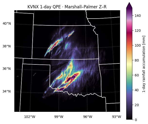
QPE accumulation map#

xradar.georeference() (applied when the sweep was pulled) turned the polar (azimuth, range) gates into Cartesian x/y coordinates about the radar, which we draw on a Lambert Conformal projection centred on KVNX. The colormap starts at 0 mm so the storm structure stays legible against a black background.

/home/runner/work/radar-datatree/radar-datatree/.venv/lib/python3.12/site-packages/cartopy/mpl/geoaxes.py:1762: UserWarning: The input coordinates to pcolormesh are interpreted as cell centers, but are not monotonically increasing or decreasing. This may lead to incorrectly calculated cell edges, in which case, please supply explicit cell edges to pcolormesh.
  result = super().pcolormesh(*args, **kwargs)

/home/runner/work/radar-datatree/radar-datatree/.venv/lib/python3.12/site-packages/cartopy/io/__init__.py:242: DownloadWarning: Downloading: https://naturalearth.s3.amazonaws.com/10m_cultural/ne_10m_admin_1_states_provinces_lakes.zip
  warnings.warn(f'Downloading: {url}', DownloadWarning)

/home/runner/work/radar-datatree/radar-datatree/.venv/lib/python3.12/site-packages/cartopy/io/__init__.py:242: DownloadWarning: Downloading: https://naturalearth.s3.amazonaws.com/10m_physical/ne_10m_coastline.zip
  warnings.warn(f'Downloading: {url}', DownloadWarning)

/home/runner/work/radar-datatree/radar-datatree/.venv/lib/python3.12/site-packages/cartopy/io/__init__.py:242: DownloadWarning: Downloading: https://naturalearth.s3.amazonaws.com/10m_physical/ne_10m_lakes.zip
  warnings.warn(f'Downloading: {url}', DownloadWarning)

_images/27429ca520ee7ed79bbd047e6d5311a7ca16b57ab66f51770a81bd2533991837.png

Scaling beyond a single day — cluster recommended#

The same code path scales to longer windows just by widening the time slice. The ARCO bytes you stream grow linearly with window length; the file-based path grows linearly with the file count and saturates per-file network round-trips.

This section is not executed in CI

The 7-day, 30-day, and 6-month windows are presented below as copy-paste templates. The ARCO path scales to all of them, but on a laptop the longer windows are minutes-to-hours; on a Coiled (or any Dask) cluster they finish in seconds-to-minutes. The file-based comparison for the 6-month window is hours to days of serial download — depending on your bandwidth and CPU — please run it on a cluster rather than a laptop.

The blocks below mirror the code published in Ladino-Rincón et al. (2026, submitted to IEEE Transactions on Big Data) (Table 2 / Figure 8 / Figure 9).

1. Spin up a Coiled cluster (or any Dask cluster)#

The paper used 30 m71.xlarge spot workers in us-east-1, ~14 minutes total spend for the 6-month run. Substitute your own scheduler if you don’t use Coiled.

import coiled
from dask.distributed import Client

cluster = coiled.Cluster(
    n_workers=30,
    worker_cpu=4,
    worker_memory="16 GiB",
    region="us-east-1",
    spot_policy="spot_with_fallback",
    name="radar-datatree-qpe",
)
client = Client(cluster)
print(client.dashboard_link)

2. Define windows and run the ARCO QPE loop across VCPs#

For longer windows the radar cycles between VCPs (e.g., VCP-12 in steady precip, VCP-212 in rapid-scan severe weather), so each window needs its own cross-VCP stitch. Window first, then concatenate — assembling the whole archive up front does not scale.

Important

Reopen the tree with chunks={"vcp_time": 100} for this section. The live 1-day cell above uses the native one-scan-per-chunk layout, which is fine for ~200 scans; at the ~45,000 scans of the 6-month window it would build a task graph of tens of thousands of single-scan chunks and the sortby inside concat_sweep would crawl. Grouping 100 scans per chunk moves the same bytes with ~100× fewer tasks.

dtree = xr.open_datatree(
    session.store,
    engine="rustytree",
    group_filter=f"/*/{TARGET_SWEEP}",
    chunks={"vcp_time": 100},
)


def concat_sweep(dtree, sweep="sweep_0", dim="vcp_time"):
    """Stitch one sweep across every VCP node into a single time-sorted Dataset."""
    sweeps = [
        child[sweep].to_dataset(inherit="all_coords")
        for name, child in dtree.children.items()
        if name.startswith("VCP-")
        and sweep in child.children
        and child[sweep].sizes.get(dim, 0)
    ]
    # join="exact" instead of the default "outer": if a future VCP ever carries a
    # different azimuth or range grid, raise rather than silently NaN-padding.
    return xr.concat(
        sweeps,
        dim=dim,
        join="exact",
        coords="minimal",
        data_vars="minimal",
        compat="override",
    ).sortby(dim)


WINDOWS = {
    "1d":   ("2011-05-20 00:00", "2011-05-20 23:59"),
    "7d":   ("2011-05-20 00:00", "2011-05-26 23:59"),
    "30d":  ("2011-05-01 00:00", "2011-05-30 23:59"),
    "6mo":  ("2011-04-01 00:00", "2011-09-30 23:59"),
}

results = {}
for name, (start, end) in WINDOWS.items():
    t0 = time.time()
    dt_window = dtree.sel(vcp_time=slice(start, end)).prune(drop_size_zero_vars=True)
    ds_window = concat_sweep(dt_window, sweep=TARGET_SWEEP)
    dbzh = ds_window["DBZH"]
    depth = rain_depth(dbzh)
    accum = depth.sum("vcp_time").compute()
    elapsed = time.time() - t0

    accum.to_zarr(f"qpe_accumulation/{name}.zarr", mode="w")
    results[name] = {
        "total_time": elapsed,
        "n_timesteps": ds_window.sizes["vcp_time"],
        "useful_data_mb": dbzh.nbytes / 1024**2,
    }
    print(f"{name:>4s}: {elapsed:7.1f}s, {results[name]['n_timesteps']:>6} scans")

Measured ARCO times on the paper’s 30-worker cluster:

Window	ARCO time	Scans
1 day	~25 s	~250
7 days	~50 s	~1,800
30 days	~3 min	~7,500
6 months	~15 min	~45,000

3. File-based comparison (do not run on a laptop for 30d/6mo)#

6-month file-based: hours to days

Serial download + decode of every NEXRAD Level II file in a 6-month window can take hours to days on a laptop, depending on your bandwidth, CPU, and how far away the bucket is from your machine. On the paper’s 30-worker cluster (parallel downloads, m71.xlarge, us-east-1) the same loop finishes in minutes. The point of running this isn’t the wait — it’s to publish the speedup ratio on hardware you control.

This template needs list_nexrad_files and download_nexrad. Both are defined in full in Notebook 3 under Approach 1 — copy those two functions into your session first; they are ~35 lines and depend only on fsspec and xradar.

# Hardcoded measurements from the paper's run, so you don't have to repeat:
MEASURED_TRADITIONAL = {
    "1d":   {"total_time":   468, "n_files":   250, "total_mb":   3_700},
    "7d":   {"total_time": 2_069, "n_files": 1_800, "total_mb":  27_500},
    "30d":  {"total_time": 6_883, "n_files": 7_500, "total_mb": 113_000},
    "6mo":  {"total_time": 36_003, "n_files": 45_000, "total_mb": 670_000},
}

# To re-measure for a single window, the per-file loop is:
files = list_nexrad_files(RADAR, START, END)
trad_t0 = time.time()
sweep_dsets = []
for f in files:
    dtree_single, _ = download_nexrad(f["path"])
    ds = dtree_single[TARGET_SWEEP].ds.load()
    sweep_dsets.append(ds.expand_dims({"vcp_time": [ds.time.values[0]]}))
ds_trad = xr.concat(sweep_dsets, dim="vcp_time")
accum_trad = rain_depth(ds_trad["DBZH"]).sum("vcp_time").compute()
trad_total = time.time() - trad_t0

4. Wall-clock and throughput scaling figures#

The two scaling figures from the paper compare ARCO and file-based total wall-clock and effective throughput across the four windows on log-log axes. Window lengths are derived from WINDOWS rather than retyped, so they cannot drift from the windows actually run.

import pandas as pd

windows_h = {
    name: (pd.Timestamp(end) - pd.Timestamp(start)) / pd.Timedelta(hours=1)
    for name, (start, end) in WINDOWS.items()
}

fig, (ax_time, ax_thrpt) = plt.subplots(1, 2, figsize=(11, 4.5))

x = list(windows_h.values())
arco_t  = [results[w]["total_time"] for w in windows_h]
trad_t  = [MEASURED_TRADITIONAL[w]["total_time"] for w in windows_h]
useful  = [results[w]["useful_data_mb"] for w in windows_h]

ax_time.loglog(x, trad_t, "o-", label="Traditional (file-based)")
ax_time.loglog(x, arco_t, "o-", label="ARCO streaming")
ax_time.set_xlabel("Window length (hours, log scale)")
ax_time.set_ylabel("Wall-clock (seconds, log scale)")
ax_time.legend()
ax_time.grid(True, which="both", alpha=0.3)

ax_thrpt.loglog(x, [u/t for u, t in zip(useful, trad_t)], "o-", label="Traditional")
ax_thrpt.loglog(x, [u/t for u, t in zip(useful, arco_t)], "o-", label="ARCO streaming")
ax_thrpt.set_xlabel("Window length (hours, log scale)")
ax_thrpt.set_ylabel("Effective throughput (MB/s, log scale)")
ax_thrpt.legend()
ax_thrpt.grid(True, which="both", alpha=0.3)
plt.tight_layout()

# Speedup per window, computed from the two tables above rather than quoted.
for w in windows_h:
    print(f"{w:>4s}: {MEASURED_TRADITIONAL[w]['total_time'] / results[w]['total_time']:.0f}× faster")

← Notebook 3 — QVP Workflow Comparison · Back to Notebook 1

References#

Abernathey, R.P. et al. (2021). Cloud-Native Repositories for Big Scientific Data. Computing in Science & Engineering, 23, 26–35. https://doi.org/10.1109/MCSE.2021.3059437
Ladino-Rincón, A., et al. (2026). Radar DataTree: A Cloud-Native AI-Ready Data Model for Accessible, Time-Aware Weather Radar Datasets. Submitted to IEEE Transactions on Big Data.
Earlier preprint: arXiv:2510.24943, https://doi.org/10.48550/arXiv.2510.24943
Marshall, J.S. & Palmer, W.M. (1948). The distribution of raindrops with size. J. Meteor., 5, 165–166.