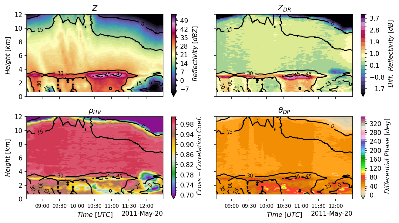
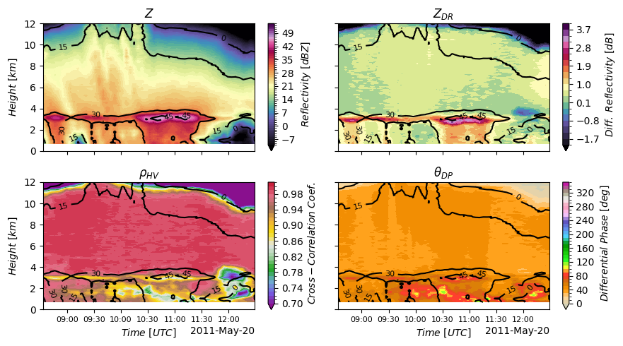
Figure 4 of Ryzhkov et al. (2016) — time-height QVP cross-sections of \(Z\), \(Z_{DR}\), \(\rho_{HV}\), and \(\Phi_{DP}\) for the May 20, 2011 KVNX MCS. This is the figure the notebook reproduces.

QVP Analysis: Traditional vs ARCO Workflows

This notebook reproduces Figure 4 from Ryzhkov et al. (2016) two ways — the traditional file-based workflow and the Analysis-Ready Cloud-Optimized (ARCO) path on s3://nexrad-arco/KVNX — then asserts the results agree to floating-point precision so the speedup is honest rather than apples-to-oranges.

Scientific goal: compute Quasi-Vertical Profiles of \(Z\), \(Z_{DR}\), \(\rho_{HV}\), and \(\Phi_{DP}\) for the May 20, 2011 MCS observed by KVNX during MC3E.

TL;DR

Reproduce Ryzhkov et al. (2016) Fig. 4 on a laptop — hours of downloading and decoding 55 NEXRAD Level II files become seconds of analysis, reading a fraction of the bytes. The notebook computes the QVP both ways and asserts numerical equivalence between them, so the speedup isn’t a different result — it’s the same result, faster.

The numbers below are measured on your machine as this notebook runs; treat them as the answer, not any figure quoted elsewhere. The file-based path is network-bound, so the ratio varies substantially between runs and machines. The data comparison is of decoded bytes and assumes a nominal 4:1 Level II compression ratio; on the wire the saving is smaller.

---

Prerequisites

This notebook assumes familiarity with the basics covered in Notebook 1 — Open NEXRAD radar archives in 5 lines with radar-datatree:

• Connecting to cloud storage with Icechunk

• Opening a DataTree with engine="rustytree"

• Time-based selection with .sel()

If you’re new to radar-datatree, start there first.

What is a Quasi-Vertical Profile (QVP)?

A Quasi-Vertical Profile (QVP) averages a polarimetric radar variable over all 360° of azimuth at a fixed high elevation (here, 19.5°), collapsing it into a time-height view of the column above the radar:

\[\text{QVP}(r, t) = \frac{1}{N_{\theta}} \sum_{\theta=0}^{360°} Z(r, \theta, t)\]

where \(r\) becomes height after the elevation correction, \(\theta\) is azimuth, and \(t\) is time.

This lets you watch the melting layer, dendritic growth zones, and aggregation signatures evolve through a storm — the killer use case Ryzhkov et al. (2016) introduce. The hero figure at the top is exactly what we’ll reproduce.

Study Parameters

We’ll analyze an expanded time window to capture more storm evolution:

• Radar: KVNX (Vance Air Force Base, Oklahoma)

• Date: May 20, 2011 (MC3E field campaign)

• Time Window: 08:30 - 12:30 UTC (4 hours)

• Elevation: 19.5° (highest WSR-88D elevation, sweep_16)

• Variables: DBZH, ZDR, RHOHV, PHIDP

import time
import tracemalloc
import warnings
from datetime import datetime, timedelta

warnings.filterwarnings("ignore", category=FutureWarning)

import cmweather  # noqa: F401  — registers ChaseSpectral / Carbone11 / PD17
import fsspec
import icechunk as ic
import matplotlib.pyplot as plt
import numpy as np
import pandas as pd
import xarray as xr
import xradar as xd

# Study parameters — expanded time window (4 hours)
RADAR = "KVNX"
START_TIME = "2011-05-20 08:30"
END_TIME = "2011-05-20 12:30"
VARIABLES = ["DBZH", "ZDR", "RHOHV", "PHIDP"]
# 19.5° elevation, the angle Ryzhkov et al. (2016) use for QVPs. Both
# the file-based loop below and the ARCO path target this exact sweep
# so they're guaranteed to operate on identical underlying scans.
SELECTED_SWEEP = "sweep_16"
# A VCP-12 NEXRAD Level II volume holds 17 sweeps and ~8 variables; the QVP
# uses one sweep and 4 variables, so the file path discards the rest.
N_TOTAL_SWEEPS = 17
N_TOTAL_VARS = 8

metrics = {"traditional": {}, "arco": {}}

Show code cell source

Hide code cell source

def list_nexrad_files(radar, start_time, end_time):
    """NEXRAD Level II objects for a radar and UTC window, oldest first."""
    start = datetime.strptime(start_time, "%Y-%m-%d %H:%M")
    end = datetime.strptime(end_time, "%Y-%m-%d %H:%M")
    fs = fsspec.filesystem("s3", anon=True)

    files, day = [], start
    while day <= end:
        try:
            listing = fs.ls(
                f"unidata-nexrad-level2/{day:%Y/%m/%d}/{radar}", detail=True
            )
        except FileNotFoundError:
            listing = []
        for info in listing:
            name = info["name"].split("/")[-1]
            if not name.startswith(radar):
                continue
            try:
                stamp = datetime.strptime(
                    name[len(radar) : len(radar) + 15], "%Y%m%d_%H%M%S"
                )
            except ValueError:
                continue  # sidecar/index objects that aren't a volume
            if start <= stamp <= end:
                files.append(
                    {
                        "path": f"s3://{info['name']}",
                        "size": info.get("size", 0),
                        "time": stamp,
                    }
                )
        day += timedelta(days=1)
    return sorted(files, key=lambda f: f["time"])


def download_nexrad(path):
    """Download and decode one Level II object -> (DataTree, compressed bytes)."""
    fs = fsspec.filesystem("s3", anon=True)
    size = fs.info(path.replace("s3://", "")).get("size", 0)
    compression = "gzip" if path.endswith(".gz") else None
    with fsspec.open(path, mode="rb", compression=compression, anon=True) as stream:
        return xd.io.open_nexradlevel2_datatree(stream.read()), size

def compute_qvp(ds, var="DBZH"):
    """Azimuthal mean of `var` as a time-height profile.

    dB-scaled variables are averaged in linear units and converted back, and
    range is projected onto height using the sweep's fixed elevation angle.
    """
    if ds[var].attrs["units"].startswith("dB"):
        qvp = 10 * np.log10((10 ** (ds[var] / 10)).mean("azimuth", skipna=True))
    else:
        qvp = ds[var].mean("azimuth", skipna=True)

    elevation = ds.sweep_fixed_angle.mean(skipna=True).values
    height = qvp.range.values * np.sin(np.deg2rad(elevation)) / 1000
    return (
        qvp.assign_coords(range=height).rename({"range": "height"}).rename(f"qvp_{var}")
    )

---

Approach 1 — Traditional file-based workflow

Discover the files, download each compressed Level II, decode it, extract the 19.5° sweep, concatenate the per-file sweeps along time, compute QVPs. Every stage blocks the next; nothing streams. This is the work the cloud-native path eliminates.

t0 = time.time()
nexrad_files = list_nexrad_files(RADAR, START_TIME, END_TIME)
metrics["traditional"]["discovery_time"] = time.time() - t0
metrics["traditional"]["total_size_mb"] = sum(f["size"] for f in nexrad_files) / 1024**2

print(
    f"Found {len(nexrad_files)} files · "
    f"{metrics['traditional']['total_size_mb']:.1f} MB compressed · "
    f"discovered in {metrics['traditional']['discovery_time']:.2f}s"
)
print(f"First: {nexrad_files[0]['path'].split('/')[-1]}")
print(f"Last:  {nexrad_files[-1]['path'].split('/')[-1]}")

Found 55 files · 808.9 MB compressed · discovered in 1.08s
First: KVNX20110520_083314_V06.gz
Last:  KVNX20110520_122911_V06.gz

# Download every file, decode it, extract SELECTED_SWEEP, hold the sweep
# datasets in RAM for later concat. tracemalloc captures the peak — the
# RAM claim downstream is grounded in this measurement.
t0 = time.time()
tracemalloc.start()

sweep_datasets = []
bytes_downloaded = 0

for file_info in nexrad_files:
    dtree_single, size_bytes = download_nexrad(file_info["path"])
    bytes_downloaded += size_bytes

    # KeyError here is intentional — silently averaging across the wrong
    # elevation would corrupt the QVP without anyone noticing.
    ds = dtree_single[SELECTED_SWEEP].ds.load()
    sweep_datasets.append(ds.expand_dims({"vcp_time": [ds.time.values[0]]}))

_, peak_mem = tracemalloc.get_traced_memory()
tracemalloc.stop()

metrics["traditional"]["total_time"] = time.time() - t0
metrics["traditional"]["files_processed"] = len(sweep_datasets)
metrics["traditional"]["peak_memory_mb"] = peak_mem / 1e6

print(
    f"Downloaded {len(sweep_datasets)} files · "
    f"{bytes_downloaded / 1e6:.0f} MB compressed · "
    f"peak {peak_mem / 1e6:.0f} MB RAM · "
    f"{metrics['traditional']['total_time']:.1f}s total"
)

Downloaded 55 files · 848 MB compressed · peak 3083 MB RAM · 274.8s total

Show code cell source

Hide code cell source

# Concatenate the per-file sweeps, then compute QVPs with the same helper
# the ARCO path uses below. Identical transforms on both sides means the
# results can be compared value-for-value (see the equivalence assertion).
t0 = time.time()
tracemalloc.start()

ds_traditional = xr.concat(sweep_datasets, dim="vcp_time")
metrics["traditional"]["concat_time"] = time.time() - t0

t0 = time.time()
qvp_traditional = {var: compute_qvp(ds_traditional, var) for var in VARIABLES}
metrics["traditional"]["qvp_compute_time"] = time.time() - t0

_, peak_mem = tracemalloc.get_traced_memory()
tracemalloc.stop()

t = metrics["traditional"]
t["concat_peak_memory_mb"] = peak_mem / 1e6
t["total_workflow_time"] = t["total_time"] + t["concat_time"] + t["qvp_compute_time"]

pd.Series(
    {
        "Files processed": t["files_processed"],
        "Download + decode [s]": round(t["total_time"], 1),
        "Concatenate [s]": round(t["concat_time"], 2),
        "QVP compute [s]": round(t["qvp_compute_time"], 2),
        "Total workflow [s]": round(t["total_workflow_time"], 1),
        "Network transfer [MB]": round(t["total_size_mb"], 1),
        "Peak RAM, download [MB]": round(t["peak_memory_mb"]),
        "Peak RAM, concat [MB]": round(t["concat_peak_memory_mb"]),
    },
    name="Traditional workflow",
).to_frame()

	Traditional workflow
Files processed	55.00
Download + decode [s]	274.80
Concatenate [s]	1.60
QVP compute [s]	1.88
Total workflow [s]	278.30
Network transfer [MB]	808.90
Peak RAM, download [MB]	3083.00
Peak RAM, concat [MB]	5793.00

---

Approach 2 — ARCO streaming

Open the Icechunk repository (metadata only), navigate to the sweep we want, slice the 4-hour window on the native vcp_time dimension. No file iteration, no decoding. Chunks stream on demand only when .compute() is called below.

Show code cell source

Hide code cell source

%%time
t0 = time.time()

storage = ic.s3_storage(
    bucket="nexrad-arco",
    prefix=RADAR,
    endpoint_url="https://umn1.osn.mghpcc.org",
    anonymous=True,
    force_path_style=True,
    region="us-east-1",
)

# Manifest tuning: split chunk manifests roughly yearly along vcp_time, and
# preload the small coordinate manifests so the first .sel() doesn't stall.
repo_config = ic.RepositoryConfig(
    manifest=ic.ManifestConfig(
        splitting=ic.ManifestSplittingConfig.from_dict(
            {
                ic.ManifestSplitCondition.AnyArray(): {
                    ic.ManifestSplitDimCondition.DimensionName("vcp_time"): 12
                    * 24
                    * 365
                }
            }
        ),
        preload=ic.ManifestPreloadConfig(
            max_total_refs=10_000,
            preload_if=ic.ManifestPreloadCondition.and_conditions(
                [
                    ic.ManifestPreloadCondition.name_matches(
                        r"^(vcp_time|azimuth|range)$"
                    ),
                    ic.ManifestPreloadCondition.num_refs(0, 10_000),
                ]
            ),
        ),
    )
)
repo = ic.Repository.open(storage, config=repo_config)
session = repo.readonly_session("main")

metrics["arco"]["connect_time"] = time.time() - t0
print(f"Connected to Icechunk repository in {metrics['arco']['connect_time']:.2f}s")

Connected to Icechunk repository in 0.66s
CPU times: user 48.9 ms, sys: 3.04 ms, total: 51.9 ms
Wall time: 663 ms

Open the radar datatree using xarray.

%%time
t0 = time.time()

# Open only the sweep we need across all VCPs. The `/*/sweep_16` glob
# trims the tree from "every VCP × every sweep" down to just SELECTED_SWEEP
# (the 19.5° elevation Ryzhkov et al. 2016 use for QVPs). See
# Notebook 1's "Opening only what you need" section for the same pattern.
dtree = xr.open_datatree(
    session.store,
    engine="rustytree",
    group_filter=f"/*/{SELECTED_SWEEP}",
    chunks={},
)

metrics["arco"]["open_datatree_time"] = time.time() - t0
print(f"Opened DataTree in {metrics['arco']['open_datatree_time']:.2f}s")

Opened DataTree in 1.25s
CPU times: user 168 ms, sys: 26.2 ms, total: 195 ms
Wall time: 1.25 s

dtree

<xarray.DataTree>
Group: /
├── Group: /VCP-12
│   │   Dimensions:        (vcp_time: 3577)
│   │   Coordinates:
│   │     * vcp_time       (vcp_time) datetime64[ns] 29kB 2011-04-08T22:31:19.547000 ...
│   │       altitude       int64 8B ...
│   │       latitude       float64 8B ...
│   │       longitude      float64 8B ...
│   │   Data variables:
│   │       volume_number  (vcp_time) float64 29kB dask.array<chunksize=(1,), meta=np.ndarray>
│   │   Attributes:
│   │       Conventions:  Cf/Radial instrument_parameters radar_parameters
│   │       attribution:  NOAA NEXRAD Level 2 data processed by Atmoscale from NOAA O...
│   │       dataset_id:   nexrad-arco-kvnx
│   │       institution:  NOAA National Weather Service
│   │       source:       WSR-88D S-band weather radar
│   │       time_domain:  2026-04-27 to Present
│   │       title:        NEXRAD ARCO - KVNX
│   │       version:      2.1
│   └── Group: /VCP-12/sweep_16
│           Dimensions:              (vcp_time: 3577, azimuth: 360, range: 460)
│           Coordinates:
│             * azimuth              (azimuth) float64 3kB 0.5 1.5 2.5 ... 357.5 358.5 359.5
│               elevation            (azimuth) float64 3kB dask.array<chunksize=(360,), meta=np.ndarray>
│               time                 (vcp_time, azimuth) datetime64[ns] 10MB dask.array<chunksize=(1, 360), meta=np.ndarray>
│             * range                (range) float32 2kB 2.125e+03 2.375e+03 ... 1.169e+05
│           Data variables:
│               CCORH                (vcp_time, azimuth, range) float32 2GB dask.array<chunksize=(1, 360, 460), meta=np.ndarray>
│               DBZH                 (vcp_time, azimuth, range) float32 2GB dask.array<chunksize=(1, 360, 460), meta=np.ndarray>
│               PHIDP                (vcp_time, azimuth, range) float32 2GB dask.array<chunksize=(1, 360, 460), meta=np.ndarray>
│               RHOHV                (vcp_time, azimuth, range) float32 2GB dask.array<chunksize=(1, 360, 460), meta=np.ndarray>
│               VRADH                (vcp_time, azimuth, range) float32 2GB dask.array<chunksize=(1, 360, 460), meta=np.ndarray>
│               WRADH                (vcp_time, azimuth, range) float32 2GB dask.array<chunksize=(1, 360, 460), meta=np.ndarray>
│               ZDR                  (vcp_time, azimuth, range) float32 2GB dask.array<chunksize=(1, 360, 460), meta=np.ndarray>
│               ray_elevation_angle  (vcp_time, azimuth) float64 10MB dask.array<chunksize=(1, 360), meta=np.ndarray>
│               sweep_fixed_angle    (vcp_time) float32 14kB dask.array<chunksize=(1,), meta=np.ndarray>
│               sweep_number         (vcp_time) float32 14kB dask.array<chunksize=(1,), meta=np.ndarray>
├── Group: /VCP-121
│   │   Dimensions:        (vcp_time: 1)
│   │   Coordinates:
│   │     * vcp_time       (vcp_time) datetime64[ns] 8B 2011-08-06T03:42:31.495000
│   │       altitude       int64 8B ...
│   │       latitude       float64 8B ...
│   │       longitude      float64 8B ...
│   │   Data variables:
│   │       volume_number  (vcp_time) float64 8B dask.array<chunksize=(1,), meta=np.ndarray>
│   │   Attributes:
│   │       Conventions:  Cf/Radial instrument_parameters radar_parameters
│   │       attribution:  NOAA NEXRAD Level 2 data processed by Atmoscale from NOAA O...
│   │       dataset_id:   nexrad-arco-kvnx
│   │       institution:  NOAA National Weather Service
│   │       source:       WSR-88D S-band weather radar
│   │       time_domain:  2026-04-27 to Present
│   │       title:        NEXRAD ARCO - KVNX
│   │       version:      2.1
│   └── Group: /VCP-121/sweep_16
│           Dimensions:              (vcp_time: 1, azimuth: 360, range: 924)
│           Coordinates:
│             * azimuth              (azimuth) float64 3kB 0.5 1.5 2.5 ... 357.5 358.5 359.5
│               elevation            (azimuth) float64 3kB dask.array<chunksize=(360,), meta=np.ndarray>
│               time                 (vcp_time, azimuth) datetime64[ns] 3kB dask.array<chunksize=(1, 360), meta=np.ndarray>
│             * range                (range) float32 4kB 2.125e+03 2.375e+03 ... 2.329e+05
│           Data variables:
│               DBZH                 (vcp_time, azimuth, range) float32 1MB dask.array<chunksize=(1, 360, 924), meta=np.ndarray>
│               PHIDP                (vcp_time, azimuth, range) float32 1MB dask.array<chunksize=(1, 360, 924), meta=np.ndarray>
│               RHOHV                (vcp_time, azimuth, range) float32 1MB dask.array<chunksize=(1, 360, 924), meta=np.ndarray>
│               VRADH                (vcp_time, azimuth, range) float32 1MB dask.array<chunksize=(1, 360, 924), meta=np.ndarray>
│               WRADH                (vcp_time, azimuth, range) float32 1MB dask.array<chunksize=(1, 360, 924), meta=np.ndarray>
│               ZDR                  (vcp_time, azimuth, range) float32 1MB dask.array<chunksize=(1, 360, 924), meta=np.ndarray>
│               ray_elevation_angle  (vcp_time, azimuth) float64 3kB dask.array<chunksize=(1, 360), meta=np.ndarray>
│               sweep_fixed_angle    (vcp_time) float32 4B dask.array<chunksize=(1,), meta=np.ndarray>
│               sweep_number         (vcp_time) float32 4B dask.array<chunksize=(1,), meta=np.ndarray>
└── Group: /VCP-212
    │   Dimensions:        (vcp_time: 748)
    │   Coordinates:
    │     * vcp_time       (vcp_time) datetime64[ns] 6kB 2011-05-20T19:19:02.487000 ....
    │       altitude       int64 8B ...
    │       latitude       float64 8B ...
    │       longitude      float64 8B ...
    │   Data variables:
    │       volume_number  (vcp_time) float64 6kB dask.array<chunksize=(1,), meta=np.ndarray>
    │   Attributes:
    │       Conventions:  Cf/Radial instrument_parameters radar_parameters
    │       attribution:  NOAA NEXRAD Level 2 data processed by Atmoscale from NOAA O...
    │       dataset_id:   nexrad-arco-kvnx
    │       institution:  NOAA National Weather Service
    │       source:       WSR-88D S-band weather radar
    │       time_domain:  2026-04-27 to Present
    │       title:        NEXRAD ARCO - KVNX
    │       version:      2.1
    └── Group: /VCP-212/sweep_16
            Dimensions:              (vcp_time: 748, azimuth: 360, range: 460)
            Coordinates:
              * azimuth              (azimuth) float64 3kB 0.5 1.5 2.5 ... 357.5 358.5 359.5
                elevation            (azimuth) float64 3kB dask.array<chunksize=(360,), meta=np.ndarray>
                time                 (vcp_time, azimuth) datetime64[ns] 2MB dask.array<chunksize=(1, 360), meta=np.ndarray>
              * range                (range) float32 2kB 2.125e+03 2.375e+03 ... 1.169e+05
            Data variables:
                CCORH                (vcp_time, azimuth, range) float32 495MB dask.array<chunksize=(1, 360, 460), meta=np.ndarray>
                DBZH                 (vcp_time, azimuth, range) float32 495MB dask.array<chunksize=(1, 360, 460), meta=np.ndarray>
                PHIDP                (vcp_time, azimuth, range) float32 495MB dask.array<chunksize=(1, 360, 460), meta=np.ndarray>
                RHOHV                (vcp_time, azimuth, range) float32 495MB dask.array<chunksize=(1, 360, 460), meta=np.ndarray>
                VRADH                (vcp_time, azimuth, range) float32 495MB dask.array<chunksize=(1, 360, 460), meta=np.ndarray>
                WRADH                (vcp_time, azimuth, range) float32 495MB dask.array<chunksize=(1, 360, 460), meta=np.ndarray>
                ZDR                  (vcp_time, azimuth, range) float32 495MB dask.array<chunksize=(1, 360, 460), meta=np.ndarray>
                ray_elevation_angle  (vcp_time, azimuth) float64 2MB dask.array<chunksize=(1, 360), meta=np.ndarray>
                sweep_fixed_angle    (vcp_time) float32 3kB dask.array<chunksize=(1,), meta=np.ndarray>
                sweep_number         (vcp_time) float32 3kB dask.array<chunksize=(1,), meta=np.ndarray>

xarray.DataTree

• /VCP-12(27)

  • /VCP-12/sweep_16(14)

    • Dimensions:
      • vcp_time: 3577
      • azimuth: 360
      • range: 460
    • Coordinates: (4)
      • azimuth
        (azimuth)
        float64
        0.5 1.5 2.5 ... 357.5 358.5 359.5

        array([  0.5,   1.5,   2.5, ..., 357.5, 358.5, 359.5], shape=(360,))

      • elevation
        (azimuth)
        float64
        dask.array<chunksize=(360,), meta=np.ndarray>

        axis :

        radial_elevation_coordinate

        long_name :

        elevation_angle_from_horizontal_plane

        standard_name :

        ray_elevation_angle

        units :

        degrees

        Array Chunk Bytes 2.81 kiB 2.81 kiB Shape (360,) (360,) Dask graph 1 chunks in 2 graph layers Data type float64 numpy.ndarray

      • time
        (vcp_time, azimuth)
        datetime64[ns]
        dask.array<chunksize=(1, 360), meta=np.ndarray>

        standard_name :

        time

        Array Chunk Bytes 9.82 MiB 2.81 kiB Shape (3577, 360) (1, 360) Dask graph 3577 chunks in 2 graph layers Data type datetime64[ns] numpy.ndarray

      • range
        (range)
        float32
        2.125e+03 2.375e+03 ... 1.169e+05

        axis :

        radial_range_coordinate

        long_name :

        range_to_measurement_volume

        meters_between_gates :

        250.0

        meters_to_center_of_first_gate :

        2125.0

        spacing_is_constant :

        true

        standard_name :

        projection_range_coordinate

        units :

        meters

        array([  2125.,   2375.,   2625., ..., 116375., 116625., 116875.],shape=(460,), dtype=float32)

    • Data variables: (10)
      • CCORH
        (vcp_time, azimuth, range)
        float32
        dask.array<chunksize=(1, 360, 460), meta=np.ndarray>

        long_name :

        Clutter Correction H

        standard_name :

        clutter_correction_h

        units :

        unitless

        Array Chunk Bytes 2.21 GiB 646.88 kiB Shape (3577, 360, 460) (1, 360, 460) Dask graph 3577 chunks in 2 graph layers Data type float32 numpy.ndarray

      • DBZH
        (vcp_time, azimuth, range)
        float32
        dask.array<chunksize=(1, 360, 460), meta=np.ndarray>

        long_name :

        Equivalent reflectivity factor H

        standard_name :

        radar_equivalent_reflectivity_factor_h

        units :

        dBZ

        Array Chunk Bytes 2.21 GiB 646.88 kiB Shape (3577, 360, 460) (1, 360, 460) Dask graph 3577 chunks in 2 graph layers Data type float32 numpy.ndarray

      • PHIDP
        (vcp_time, azimuth, range)
        float32
        dask.array<chunksize=(1, 360, 460), meta=np.ndarray>

        long_name :

        Differential phase HV

        standard_name :

        radar_differential_phase_hv

        units :

        degrees

        Array Chunk Bytes 2.21 GiB 646.88 kiB Shape (3577, 360, 460) (1, 360, 460) Dask graph 3577 chunks in 2 graph layers Data type float32 numpy.ndarray

      • RHOHV
        (vcp_time, azimuth, range)
        float32
        dask.array<chunksize=(1, 360, 460), meta=np.ndarray>

        long_name :

        Correlation coefficient HV

        standard_name :

        radar_correlation_coefficient_hv

        units :

        unitless

        Array Chunk Bytes 2.21 GiB 646.88 kiB Shape (3577, 360, 460) (1, 360, 460) Dask graph 3577 chunks in 2 graph layers Data type float32 numpy.ndarray

      • VRADH
        (vcp_time, azimuth, range)
        float32
        dask.array<chunksize=(1, 360, 460), meta=np.ndarray>

        long_name :

        Radial velocity H

        standard_name :

        radial_velocity_of_scatterers_away_from_instrument

        units :

        m/s

        Array Chunk Bytes 2.21 GiB 646.88 kiB Shape (3577, 360, 460) (1, 360, 460) Dask graph 3577 chunks in 2 graph layers Data type float32 numpy.ndarray

      • WRADH
        (vcp_time, azimuth, range)
        float32
        dask.array<chunksize=(1, 360, 460), meta=np.ndarray>

        long_name :

        Doppler spectrum width H

        standard_name :

        radar_spectrum_width

        units :

        m/s

        Array Chunk Bytes 2.21 GiB 646.88 kiB Shape (3577, 360, 460) (1, 360, 460) Dask graph 3577 chunks in 2 graph layers Data type float32 numpy.ndarray

      • ZDR
        (vcp_time, azimuth, range)
        float32
        dask.array<chunksize=(1, 360, 460), meta=np.ndarray>

        long_name :

        Log differential reflectivity H/V

        standard_name :

        radar_differential_reflectivity_hv

        units :

        dB

        Array Chunk Bytes 2.21 GiB 646.88 kiB Shape (3577, 360, 460) (1, 360, 460) Dask graph 3577 chunks in 2 graph layers Data type float32 numpy.ndarray

      • ray_elevation_angle
        (vcp_time, azimuth)
        float64
        dask.array<chunksize=(1, 360), meta=np.ndarray>

        axis :

        radial_elevation_coordinate

        long_name :

        elevation_angle_from_horizontal_plane

        standard_name :

        ray_elevation_angle

        units :

        degrees

        Array Chunk Bytes 9.82 MiB 2.81 kiB Shape (3577, 360) (1, 360) Dask graph 3577 chunks in 2 graph layers Data type float64 numpy.ndarray

      • sweep_fixed_angle
        (vcp_time)
        float32
        dask.array<chunksize=(1,), meta=np.ndarray>

        Array Chunk Bytes 13.97 kiB 4 B Shape (3577,) (1,) Dask graph 3577 chunks in 2 graph layers Data type float32 numpy.ndarray

      • sweep_number
        (vcp_time)
        float32
        dask.array<chunksize=(1,), meta=np.ndarray>

        Array Chunk Bytes 13.97 kiB 4 B Shape (3577,) (1,) Dask graph 3577 chunks in 2 graph layers Data type float32 numpy.ndarray

  • Dimensions:
    • vcp_time: 3577
  • Coordinates: (4)
    • vcp_time
      (vcp_time)
      datetime64[ns]
      2011-04-08T22:31:19.547000 ... 2...

      axis :

      T

      description :

      Volume Coverage Pattern time since start of volume scan

      long_name :

      time of volume coverage pattern scan

      standard_name :

      time

      array(['2011-04-08T22:31:19.547000000', '2011-04-08T22:35:40.841000000','2011-04-08T22:40:01.859000000', ..., '2011-09-18T11:43:51.817000000','2011-09-18T11:48:11.937000000', '2011-09-18T11:52:32.427000000'],shape=(3577,), dtype='datetime64[ns]')

    • altitude
      ()
      int64
      ...

      [1 values with dtype=int64]

    • latitude
      ()
      float64
      ...

      [1 values with dtype=float64]

    • longitude
      ()
      float64
      ...

      [1 values with dtype=float64]

  • Data variables: (1)
    • volume_number
      (vcp_time)
      float64
      dask.array<chunksize=(1,), meta=np.ndarray>

      Array Chunk Bytes 27.95 kiB 8 B Shape (3577,) (1,) Dask graph 3577 chunks in 2 graph layers Data type float64 numpy.ndarray

  • Attributes: (8)

    Conventions :

    Cf/Radial instrument_parameters radar_parameters

    attribution :

    NOAA NEXRAD Level 2 data processed by Atmoscale from NOAA Open Data Dissemination archives.

    dataset_id :

    nexrad-arco-kvnx

    institution :

    NOAA National Weather Service

    source :

    WSR-88D S-band weather radar

    time_domain :

    2026-04-27 to Present

    title :

    NEXRAD ARCO - KVNX

    version :

    2.1

  /VCP-121(26)

  • /VCP-121/sweep_16(13)

    • Dimensions:
      • vcp_time: 1
      • azimuth: 360
      • range: 924
    • Coordinates: (4)
      • azimuth
        (azimuth)
        float64
        0.5 1.5 2.5 ... 357.5 358.5 359.5

        array([  0.5,   1.5,   2.5, ..., 357.5, 358.5, 359.5], shape=(360,))

      • elevation
        (azimuth)
        float64
        dask.array<chunksize=(360,), meta=np.ndarray>

        axis :

        radial_elevation_coordinate

        long_name :

        elevation_angle_from_horizontal_plane

        standard_name :

        ray_elevation_angle

        units :

        degrees

        Array Chunk Bytes 2.81 kiB 2.81 kiB Shape (360,) (360,) Dask graph 1 chunks in 2 graph layers Data type float64 numpy.ndarray

      • time
        (vcp_time, azimuth)
        datetime64[ns]
        dask.array<chunksize=(1, 360), meta=np.ndarray>

        standard_name :

        time

        Array Chunk Bytes 2.81 kiB 2.81 kiB Shape (1, 360) (1, 360) Dask graph 1 chunks in 2 graph layers Data type datetime64[ns] numpy.ndarray

      • range
        (range)
        float32
        2.125e+03 2.375e+03 ... 2.329e+05

        axis :

        radial_range_coordinate

        long_name :

        range_to_measurement_volume

        meters_between_gates :

        250.0

        meters_to_center_of_first_gate :

        2125.0

        spacing_is_constant :

        true

        standard_name :

        projection_range_coordinate

        units :

        meters

        array([  2125.,   2375.,   2625., ..., 232375., 232625., 232875.],shape=(924,), dtype=float32)

    • Data variables: (9)
      • DBZH
        (vcp_time, azimuth, range)
        float32
        dask.array<chunksize=(1, 360, 924), meta=np.ndarray>

        long_name :

        Equivalent reflectivity factor H

        standard_name :

        radar_equivalent_reflectivity_factor_h

        units :

        dBZ

        Array Chunk Bytes 1.27 MiB 1.27 MiB Shape (1, 360, 924) (1, 360, 924) Dask graph 1 chunks in 2 graph layers Data type float32 numpy.ndarray

      • PHIDP
        (vcp_time, azimuth, range)
        float32
        dask.array<chunksize=(1, 360, 924), meta=np.ndarray>

        long_name :

        Differential phase HV

        standard_name :

        radar_differential_phase_hv

        units :

        degrees

        Array Chunk Bytes 1.27 MiB 1.27 MiB Shape (1, 360, 924) (1, 360, 924) Dask graph 1 chunks in 2 graph layers Data type float32 numpy.ndarray

      • RHOHV
        (vcp_time, azimuth, range)
        float32
        dask.array<chunksize=(1, 360, 924), meta=np.ndarray>

        long_name :

        Correlation coefficient HV

        standard_name :

        radar_correlation_coefficient_hv

        units :

        unitless

        Array Chunk Bytes 1.27 MiB 1.27 MiB Shape (1, 360, 924) (1, 360, 924) Dask graph 1 chunks in 2 graph layers Data type float32 numpy.ndarray

      • VRADH
        (vcp_time, azimuth, range)
        float32
        dask.array<chunksize=(1, 360, 924), meta=np.ndarray>

        long_name :

        Radial velocity H

        standard_name :

        radial_velocity_of_scatterers_away_from_instrument

        units :

        m/s

        Array Chunk Bytes 1.27 MiB 1.27 MiB Shape (1, 360, 924) (1, 360, 924) Dask graph 1 chunks in 2 graph layers Data type float32 numpy.ndarray

      • WRADH
        (vcp_time, azimuth, range)
        float32
        dask.array<chunksize=(1, 360, 924), meta=np.ndarray>

        long_name :

        Doppler spectrum width H

        standard_name :

        radar_spectrum_width

        units :

        m/s

        Array Chunk Bytes 1.27 MiB 1.27 MiB Shape (1, 360, 924) (1, 360, 924) Dask graph 1 chunks in 2 graph layers Data type float32 numpy.ndarray

      • ZDR
        (vcp_time, azimuth, range)
        float32
        dask.array<chunksize=(1, 360, 924), meta=np.ndarray>

        long_name :

        Log differential reflectivity H/V

        standard_name :

        radar_differential_reflectivity_hv

        units :

        dB

        Array Chunk Bytes 1.27 MiB 1.27 MiB Shape (1, 360, 924) (1, 360, 924) Dask graph 1 chunks in 2 graph layers Data type float32 numpy.ndarray

      • ray_elevation_angle
        (vcp_time, azimuth)
        float64
        dask.array<chunksize=(1, 360), meta=np.ndarray>

        axis :

        radial_elevation_coordinate

        long_name :

        elevation_angle_from_horizontal_plane

        standard_name :

        ray_elevation_angle

        units :

        degrees

        Array Chunk Bytes 2.81 kiB 2.81 kiB Shape (1, 360) (1, 360) Dask graph 1 chunks in 2 graph layers Data type float64 numpy.ndarray

      • sweep_fixed_angle
        (vcp_time)
        float32
        dask.array<chunksize=(1,), meta=np.ndarray>

        Array Chunk Bytes 4 B 4 B Shape (1,) (1,) Dask graph 1 chunks in 2 graph layers Data type float32 numpy.ndarray

      • sweep_number
        (vcp_time)
        float32
        dask.array<chunksize=(1,), meta=np.ndarray>

        Array Chunk Bytes 4 B 4 B Shape (1,) (1,) Dask graph 1 chunks in 2 graph layers Data type float32 numpy.ndarray

  • Dimensions:
    • vcp_time: 1
  • Coordinates: (4)
    • vcp_time
      (vcp_time)
      datetime64[ns]
      2011-08-06T03:42:31.495000

      axis :

      T

      description :

      Volume Coverage Pattern time since start of volume scan

      long_name :

      time of volume coverage pattern scan

      standard_name :

      time

      array(['2011-08-06T03:42:31.495000000'], dtype='datetime64[ns]')

    • altitude
      ()
      int64
      ...

      [1 values with dtype=int64]

    • latitude
      ()
      float64
      ...

      [1 values with dtype=float64]

    • longitude
      ()
      float64
      ...

      [1 values with dtype=float64]

  • Data variables: (1)
    • volume_number
      (vcp_time)
      float64
      dask.array<chunksize=(1,), meta=np.ndarray>

      Array Chunk Bytes 8 B 8 B Shape (1,) (1,) Dask graph 1 chunks in 2 graph layers Data type float64 numpy.ndarray

  • Attributes: (8)

    Conventions :

    Cf/Radial instrument_parameters radar_parameters

    attribution :

    NOAA NEXRAD Level 2 data processed by Atmoscale from NOAA Open Data Dissemination archives.

    dataset_id :

    nexrad-arco-kvnx

    institution :

    NOAA National Weather Service

    source :

    WSR-88D S-band weather radar

    time_domain :

    2026-04-27 to Present

    title :

    NEXRAD ARCO - KVNX

    version :

    2.1

  /VCP-212(27)

  • /VCP-212/sweep_16(14)

    • Dimensions:
      • vcp_time: 748
      • azimuth: 360
      • range: 460
    • Coordinates: (4)
      • azimuth
        (azimuth)
        float64
        0.5 1.5 2.5 ... 357.5 358.5 359.5

        array([  0.5,   1.5,   2.5, ..., 357.5, 358.5, 359.5], shape=(360,))

      • elevation
        (azimuth)
        float64
        dask.array<chunksize=(360,), meta=np.ndarray>

        axis :

        radial_elevation_coordinate

        long_name :

        elevation_angle_from_horizontal_plane

        standard_name :

        ray_elevation_angle

        units :

        degrees

        Array Chunk Bytes 2.81 kiB 2.81 kiB Shape (360,) (360,) Dask graph 1 chunks in 2 graph layers Data type float64 numpy.ndarray

      • time
        (vcp_time, azimuth)
        datetime64[ns]
        dask.array<chunksize=(1, 360), meta=np.ndarray>

        standard_name :

        time

        Array Chunk Bytes 2.05 MiB 2.81 kiB Shape (748, 360) (1, 360) Dask graph 748 chunks in 2 graph layers Data type datetime64[ns] numpy.ndarray

      • range
        (range)
        float32
        2.125e+03 2.375e+03 ... 1.169e+05

        axis :

        radial_range_coordinate

        long_name :

        range_to_measurement_volume

        meters_between_gates :

        250.0

        meters_to_center_of_first_gate :

        2125.0

        spacing_is_constant :

        true

        standard_name :

        projection_range_coordinate

        units :

        meters

        array([  2125.,   2375.,   2625., ..., 116375., 116625., 116875.],shape=(460,), dtype=float32)

    • Data variables: (10)
      • CCORH
        (vcp_time, azimuth, range)
        float32
        dask.array<chunksize=(1, 360, 460), meta=np.ndarray>

        long_name :

        Clutter Correction H

        standard_name :

        clutter_correction_h

        units :

        unitless

        Array Chunk Bytes 472.52 MiB 646.88 kiB Shape (748, 360, 460) (1, 360, 460) Dask graph 748 chunks in 2 graph layers Data type float32 numpy.ndarray

      • DBZH
        (vcp_time, azimuth, range)
        float32
        dask.array<chunksize=(1, 360, 460), meta=np.ndarray>

        long_name :

        Equivalent reflectivity factor H

        standard_name :

        radar_equivalent_reflectivity_factor_h

        units :

        dBZ

        Array Chunk Bytes 472.52 MiB 646.88 kiB Shape (748, 360, 460) (1, 360, 460) Dask graph 748 chunks in 2 graph layers Data type float32 numpy.ndarray

      • PHIDP
        (vcp_time, azimuth, range)
        float32
        dask.array<chunksize=(1, 360, 460), meta=np.ndarray>

        long_name :

        Differential phase HV

        standard_name :

        radar_differential_phase_hv

        units :

        degrees

        Array Chunk Bytes 472.52 MiB 646.88 kiB Shape (748, 360, 460) (1, 360, 460) Dask graph 748 chunks in 2 graph layers Data type float32 numpy.ndarray

      • RHOHV
        (vcp_time, azimuth, range)
        float32
        dask.array<chunksize=(1, 360, 460), meta=np.ndarray>

        long_name :

        Correlation coefficient HV

        standard_name :

        radar_correlation_coefficient_hv

        units :

        unitless

        Array Chunk Bytes 472.52 MiB 646.88 kiB Shape (748, 360, 460) (1, 360, 460) Dask graph 748 chunks in 2 graph layers Data type float32 numpy.ndarray

      • VRADH
        (vcp_time, azimuth, range)
        float32
        dask.array<chunksize=(1, 360, 460), meta=np.ndarray>

        long_name :

        Radial velocity H

        standard_name :

        radial_velocity_of_scatterers_away_from_instrument

        units :

        m/s

        Array Chunk Bytes 472.52 MiB 646.88 kiB Shape (748, 360, 460) (1, 360, 460) Dask graph 748 chunks in 2 graph layers Data type float32 numpy.ndarray

      • WRADH
        (vcp_time, azimuth, range)
        float32
        dask.array<chunksize=(1, 360, 460), meta=np.ndarray>

        long_name :

        Doppler spectrum width H

        standard_name :

        radar_spectrum_width

        units :

        m/s

        Array Chunk Bytes 472.52 MiB 646.88 kiB Shape (748, 360, 460) (1, 360, 460) Dask graph 748 chunks in 2 graph layers Data type float32 numpy.ndarray

      • ZDR
        (vcp_time, azimuth, range)
        float32
        dask.array<chunksize=(1, 360, 460), meta=np.ndarray>

        long_name :

        Log differential reflectivity H/V

        standard_name :

        radar_differential_reflectivity_hv

        units :

        dB

        Array Chunk Bytes 472.52 MiB 646.88 kiB Shape (748, 360, 460) (1, 360, 460) Dask graph 748 chunks in 2 graph layers Data type float32 numpy.ndarray

      • ray_elevation_angle
        (vcp_time, azimuth)
        float64
        dask.array<chunksize=(1, 360), meta=np.ndarray>

        axis :

        radial_elevation_coordinate

        long_name :

        elevation_angle_from_horizontal_plane

        standard_name :

        ray_elevation_angle

        units :

        degrees

        Array Chunk Bytes 2.05 MiB 2.81 kiB Shape (748, 360) (1, 360) Dask graph 748 chunks in 2 graph layers Data type float64 numpy.ndarray

      • sweep_fixed_angle
        (vcp_time)
        float32
        dask.array<chunksize=(1,), meta=np.ndarray>

        Array Chunk Bytes 2.92 kiB 4 B Shape (748,) (1,) Dask graph 748 chunks in 2 graph layers Data type float32 numpy.ndarray

      • sweep_number
        (vcp_time)
        float32
        dask.array<chunksize=(1,), meta=np.ndarray>

        Array Chunk Bytes 2.92 kiB 4 B Shape (748,) (1,) Dask graph 748 chunks in 2 graph layers Data type float32 numpy.ndarray

  • Dimensions:
    • vcp_time: 748
  • Coordinates: (4)
    • vcp_time
      (vcp_time)
      datetime64[ns]
      2011-05-20T19:19:02.487000 ... 2...

      axis :

      T

      description :

      Volume Coverage Pattern time since start of volume scan

      long_name :

      time of volume coverage pattern scan

      standard_name :

      time

      array(['2011-05-20T19:19:02.487000000', '2011-05-20T19:23:43.749000000','2011-05-20T19:28:26.192000000', ..., '2011-08-13T02:05:39.624000000','2011-08-13T02:10:20.078000000', '2011-08-13T02:15:00.456000000'],shape=(748,), dtype='datetime64[ns]')

    • altitude
      ()
      int64
      ...

      [1 values with dtype=int64]

    • latitude
      ()
      float64
      ...

      [1 values with dtype=float64]

    • longitude
      ()
      float64
      ...

      [1 values with dtype=float64]

  • Data variables: (1)
    • volume_number
      (vcp_time)
      float64
      dask.array<chunksize=(1,), meta=np.ndarray>

      Array Chunk Bytes 5.84 kiB 8 B Shape (748,) (1,) Dask graph 748 chunks in 2 graph layers Data type float64 numpy.ndarray

  • Attributes: (8)

    Conventions :

    Cf/Radial instrument_parameters radar_parameters

    attribution :

    NOAA NEXRAD Level 2 data processed by Atmoscale from NOAA Open Data Dissemination archives.

    dataset_id :

    nexrad-arco-kvnx

    institution :

    NOAA National Weather Service

    source :

    WSR-88D S-band weather radar

    time_domain :

    2026-04-27 to Present

    title :

    NEXRAD ARCO - KVNX

    version :

    2.1

list(dtree.children)

['VCP-12', 'VCP-121', 'VCP-212']

Each VCP’s sweep_16 is the 19.5° elevation cut. The QVP-target VCP for the May 2011 KVNX MCS is VCP-12 (precipitation mode); pull its sweep directly:

# Select the 4-hour time window
# With ARCO format, this is a simple slice operation - no file iteration needed
ds_qvp_selected = (
    dtree.sel(vcp_time=slice(START_TIME, END_TIME))
    .prune(drop_size_zero_vars=True)[f"/VCP-12/{SELECTED_SWEEP}"]
    .to_dataset()
)


ds_qvp_selected

<xarray.Dataset> Size: 255MB
Dimensions:              (vcp_time: 55, azimuth: 360, range: 460)
Coordinates:
  * vcp_time             (vcp_time) datetime64[ns] 440B 2011-05-20T08:33:14.1...
  * azimuth              (azimuth) float64 3kB 0.5 1.5 2.5 ... 357.5 358.5 359.5
    elevation            (azimuth) float64 3kB dask.array<chunksize=(360,), meta=np.ndarray>
    time                 (vcp_time, azimuth) datetime64[ns] 158kB dask.array<chunksize=(1, 360), meta=np.ndarray>
  * range                (range) float32 2kB 2.125e+03 2.375e+03 ... 1.169e+05
Data variables:
    CCORH                (vcp_time, azimuth, range) float32 36MB dask.array<chunksize=(1, 360, 460), meta=np.ndarray>
    DBZH                 (vcp_time, azimuth, range) float32 36MB dask.array<chunksize=(1, 360, 460), meta=np.ndarray>
    PHIDP                (vcp_time, azimuth, range) float32 36MB dask.array<chunksize=(1, 360, 460), meta=np.ndarray>
    RHOHV                (vcp_time, azimuth, range) float32 36MB dask.array<chunksize=(1, 360, 460), meta=np.ndarray>
    VRADH                (vcp_time, azimuth, range) float32 36MB dask.array<chunksize=(1, 360, 460), meta=np.ndarray>
    WRADH                (vcp_time, azimuth, range) float32 36MB dask.array<chunksize=(1, 360, 460), meta=np.ndarray>
    ZDR                  (vcp_time, azimuth, range) float32 36MB dask.array<chunksize=(1, 360, 460), meta=np.ndarray>
    ray_elevation_angle  (vcp_time, azimuth) float64 158kB dask.array<chunksize=(1, 360), meta=np.ndarray>
    sweep_fixed_angle    (vcp_time) float32 220B dask.array<chunksize=(1,), meta=np.ndarray>
    sweep_number         (vcp_time) float32 220B dask.array<chunksize=(1,), meta=np.ndarray>

xarray.Dataset

• Dimensions:
  • vcp_time: 55
  • azimuth: 360
  • range: 460
• Coordinates: (5)
  • vcp_time
    (vcp_time)
    datetime64[ns]
    2011-05-20T08:33:14.127000 ... 2...

    axis :

    T

    description :

    Volume Coverage Pattern time since start of volume scan

    long_name :

    time of volume coverage pattern scan

    standard_name :

    time

    array(['2011-05-20T08:33:14.127000000', '2011-05-20T08:37:34.426000000',
           '2011-05-20T08:41:53.574000000', '2011-05-20T08:46:12.952000000',
           '2011-05-20T08:50:33.364000000', '2011-05-20T08:54:53.608000000',
           '2011-05-20T08:59:12.789000000', '2011-05-20T09:03:33.061000000',
           '2011-05-20T09:07:53.203000000', '2011-05-20T09:12:12.400000000',
           '2011-05-20T09:16:32.837000000', '2011-05-20T09:20:52.255000000',
           '2011-05-20T09:27:09.585000000', '2011-05-20T09:31:28.788000000',
           '2011-05-20T09:35:48.134000000', '2011-05-20T09:40:09.521000000',
           '2011-05-20T09:44:29.563000000', '2011-05-20T09:48:49.046000000',
           '2011-05-20T09:53:08.262000000', '2011-05-20T09:57:27.484000000',
           '2011-05-20T10:01:47.882000000', '2011-05-20T10:06:08.216000000',
           '2011-05-20T10:10:28.356000000', '2011-05-20T10:14:47.812000000',
           '2011-05-20T10:19:06.937000000', '2011-05-20T10:23:27.361000000',
           '2011-05-20T10:27:47.763000000', '2011-05-20T10:32:07.679000000',
           '2011-05-20T10:36:28.128000000', '2011-05-20T10:40:47.402000000',
           '2011-05-20T10:45:07.823000000', '2011-05-20T10:49:28.114000000',
           '2011-05-20T10:53:49.401000000', '2011-05-20T10:58:09.725000000',
           '2011-05-20T11:02:30.828000000', '2011-05-20T11:06:51.182000000',
           '2011-05-20T11:11:11.450000000', '2011-05-20T11:15:30.806000000',
           '2011-05-20T11:19:51.130000000', '2011-05-20T11:24:10.404000000',
           '2011-05-20T11:28:30.608000000', '2011-05-20T11:32:51.004000000',
           '2011-05-20T11:37:10.304000000', '2011-05-20T11:41:30.595000000',
           '2011-05-20T11:45:50.924000000', '2011-05-20T11:50:11.097000000',
           '2011-05-20T11:54:31.576000000', '2011-05-20T11:58:51.755000000',
           '2011-05-20T12:03:11.035000000', '2011-05-20T12:07:31.258000000',
           '2011-05-20T12:11:50.592000000', '2011-05-20T12:16:11.898000000',
           '2011-05-20T12:20:30.806000000', '2011-05-20T12:24:52.272000000',
           '2011-05-20T12:29:11.734000000'], dtype='datetime64[ns]')

  • azimuth
    (azimuth)
    float64
    0.5 1.5 2.5 ... 357.5 358.5 359.5

    array([  0.5,   1.5,   2.5, ..., 357.5, 358.5, 359.5], shape=(360,))

  • elevation
    (azimuth)
    float64
    dask.array<chunksize=(360,), meta=np.ndarray>

    axis :

    radial_elevation_coordinate

    long_name :

    elevation_angle_from_horizontal_plane

    standard_name :

    ray_elevation_angle

    units :

    degrees

    Array Chunk Bytes 2.81 kiB 2.81 kiB Shape (360,) (360,) Dask graph 1 chunks in 2 graph layers Data type float64 numpy.ndarray

  • time
    (vcp_time, azimuth)
    datetime64[ns]
    dask.array<chunksize=(1, 360), meta=np.ndarray>

    standard_name :

    time

    Array Chunk Bytes 154.69 kiB 2.81 kiB Shape (55, 360) (1, 360) Dask graph 55 chunks in 3 graph layers Data type datetime64[ns] numpy.ndarray

  • range
    (range)
    float32
    2.125e+03 2.375e+03 ... 1.169e+05

    axis :

    radial_range_coordinate

    long_name :

    range_to_measurement_volume

    meters_between_gates :

    250.0

    meters_to_center_of_first_gate :

    2125.0

    spacing_is_constant :

    true

    standard_name :

    projection_range_coordinate

    units :

    meters

    array([  2125.,   2375.,   2625., ..., 116375., 116625., 116875.],
          shape=(460,), dtype=float32)

• Data variables: (10)
  • CCORH
    (vcp_time, azimuth, range)
    float32
    dask.array<chunksize=(1, 360, 460), meta=np.ndarray>

    long_name :

    Clutter Correction H

    standard_name :

    clutter_correction_h

    units :

    unitless

    Array Chunk Bytes 34.74 MiB 646.88 kiB Shape (55, 360, 460) (1, 360, 460) Dask graph 55 chunks in 3 graph layers Data type float32 numpy.ndarray

  • DBZH
    (vcp_time, azimuth, range)
    float32
    dask.array<chunksize=(1, 360, 460), meta=np.ndarray>

    long_name :

    Equivalent reflectivity factor H

    standard_name :

    radar_equivalent_reflectivity_factor_h

    units :

    dBZ

    Array Chunk Bytes 34.74 MiB 646.88 kiB Shape (55, 360, 460) (1, 360, 460) Dask graph 55 chunks in 3 graph layers Data type float32 numpy.ndarray

  • PHIDP
    (vcp_time, azimuth, range)
    float32
    dask.array<chunksize=(1, 360, 460), meta=np.ndarray>

    long_name :

    Differential phase HV

    standard_name :

    radar_differential_phase_hv

    units :

    degrees

    Array Chunk Bytes 34.74 MiB 646.88 kiB Shape (55, 360, 460) (1, 360, 460) Dask graph 55 chunks in 3 graph layers Data type float32 numpy.ndarray

  • RHOHV
    (vcp_time, azimuth, range)
    float32
    dask.array<chunksize=(1, 360, 460), meta=np.ndarray>

    long_name :

    Correlation coefficient HV

    standard_name :

    radar_correlation_coefficient_hv

    units :

    unitless

    Array Chunk Bytes 34.74 MiB 646.88 kiB Shape (55, 360, 460) (1, 360, 460) Dask graph 55 chunks in 3 graph layers Data type float32 numpy.ndarray

  • VRADH
    (vcp_time, azimuth, range)
    float32
    dask.array<chunksize=(1, 360, 460), meta=np.ndarray>

    long_name :

    Radial velocity H

    standard_name :

    radial_velocity_of_scatterers_away_from_instrument

    units :

    m/s

    Array Chunk Bytes 34.74 MiB 646.88 kiB Shape (55, 360, 460) (1, 360, 460) Dask graph 55 chunks in 3 graph layers Data type float32 numpy.ndarray

  • WRADH
    (vcp_time, azimuth, range)
    float32
    dask.array<chunksize=(1, 360, 460), meta=np.ndarray>

    long_name :

    Doppler spectrum width H

    standard_name :

    radar_spectrum_width

    units :

    m/s

    Array Chunk Bytes 34.74 MiB 646.88 kiB Shape (55, 360, 460) (1, 360, 460) Dask graph 55 chunks in 3 graph layers Data type float32 numpy.ndarray

  • ZDR
    (vcp_time, azimuth, range)
    float32
    dask.array<chunksize=(1, 360, 460), meta=np.ndarray>

    long_name :

    Log differential reflectivity H/V

    standard_name :

    radar_differential_reflectivity_hv

    units :

    dB

    Array Chunk Bytes 34.74 MiB 646.88 kiB Shape (55, 360, 460) (1, 360, 460) Dask graph 55 chunks in 3 graph layers Data type float32 numpy.ndarray

  • ray_elevation_angle
    (vcp_time, azimuth)
    float64
    dask.array<chunksize=(1, 360), meta=np.ndarray>

    axis :

    radial_elevation_coordinate

    long_name :

    elevation_angle_from_horizontal_plane

    standard_name :

    ray_elevation_angle

    units :

    degrees

    Array Chunk Bytes 154.69 kiB 2.81 kiB Shape (55, 360) (1, 360) Dask graph 55 chunks in 3 graph layers Data type float64 numpy.ndarray

  • sweep_fixed_angle
    (vcp_time)
    float32
    dask.array<chunksize=(1,), meta=np.ndarray>

    Array Chunk Bytes 220 B 4 B Shape (55,) (1,) Dask graph 55 chunks in 3 graph layers Data type float32 numpy.ndarray

  • sweep_number
    (vcp_time)
    float32
    dask.array<chunksize=(1,), meta=np.ndarray>

    Array Chunk Bytes 220 B 4 B Shape (55,) (1,) Dask graph 55 chunks in 3 graph layers Data type float32 numpy.ndarray

Show code cell source

Hide code cell source

# What the ARCO path actually streams: one chunk per scan, per variable.
# This dataset is stored uncompressed, so bytes on the wire == bytes in RAM.
chunks = pd.DataFrame(
    {
        var: {
            "chunks": da.data.npartitions,
            "chunk [MB]": da.dtype.itemsize * int(np.prod(da.data.chunksize)) / 1e6,
            "total [MB]": da.nbytes / 1e6,
        }
        for var, da in ((v, ds_qvp_selected[v]) for v in VARIABLES)
    }
).T

metrics["arco"]["uncompressed_mb"] = float(chunks["total [MB]"].sum())
# The file path decompresses whole volumes — every sweep, every variable.
# NEXRAD Level II gzips at roughly 4:1.
metrics["traditional"]["uncompressed_mb"] = (
    metrics["traditional"]["total_size_mb"] * 4.0
)

print(
    f"ARCO streams {int(chunks['chunks'].sum())} chunks = "
    f"{metrics['arco']['uncompressed_mb']:.1f} MB, against "
    f"{metrics['traditional']['total_size_mb']:.0f} MB downloaded / "
    f"{metrics['traditional']['uncompressed_mb']:.0f} MB decompressed by the file path."
)
chunks

ARCO streams 220 chunks = 145.7 MB, against 809 MB downloaded / 3236 MB decompressed by the file path.

	chunks	chunk [MB]	total [MB]
DBZH	55.0	0.6624	36.432
ZDR	55.0	0.6624	36.432
RHOHV	55.0	0.6624	36.432
PHIDP	55.0	0.6624	36.432

%%time
t0 = time.time()

# Vectorized across all timesteps; chunks stream on demand here.
qvp_data = {var: compute_qvp(ds_qvp_selected, var).compute() for var in VARIABLES}

a = metrics["arco"]
a["qvp_compute_time"] = time.time() - t0
a["timesteps"] = len(ds_qvp_selected.vcp_time)
a["total_time"] = a["connect_time"] + a["open_datatree_time"] + a["qvp_compute_time"]

print(
    f"Computed {len(qvp_data)} QVPs over {a['timesteps']} timesteps in "
    f"{a['qvp_compute_time']:.1f}s ({a['total_time']:.1f}s including connect + open)"
)

Computed 4 QVPs over 55 timesteps in 9.2s (11.1s including connect + open)
CPU times: user 1.6 s, sys: 67.7 ms, total: 1.67 s
Wall time: 9.2 s

Sanity check: traditional and ARCO QVPs agree

Both paths read the same sweep_16 bytes and pass them through the same compute_qvp helper, so the resulting QVPs should match within floating-point noise. This block enforces the equivalence directly — if either workflow drifted (e.g., a misaligned time slice, a chunk-decoding bug, a unit handling regression), the assertion fires.

Show code cell source

Hide code cell source

TOLERANCES = {"DBZH": 0.1, "ZDR": 0.1, "RHOHV": 0.05, "PHIDP": 0.5}

# The two paths timestamp the same scan differently: the file path uses
# sweep_16's first ray, the ARCO path the volume's vcp_time. sweep_16 is the
# last (19.5°) cut in the volume, so the file path runs ~4 min later. The
# comparison is therefore positional — but only after proving the pairs really
# are the same scans: every offset must sit in one tight band. An off-by-one
# would throw one pair a whole volume period out and blow the spread check.
VOLUME_PERIOD = np.timedelta64(6, "m")
MAX_LAG_SPREAD = np.timedelta64(60, "s")


def assert_scans_correspond():
    lhs, rhs = qvp_traditional["DBZH"], qvp_data["DBZH"]
    assert lhs.sizes == rhs.sizes, f"scan counts differ: {lhs.sizes} vs {rhs.sizes}"

    offsets = lhs.vcp_time.values - rhs.vcp_time.values
    # Bind the conditions first: a long `assert cond, msg` is the one construct
    # black and ruff-format wrap differently, so CI can never satisfy both.
    in_band = (offsets >= np.timedelta64(0)).all() and (offsets < VOLUME_PERIOD).all()
    assert in_band, f"scan pairing is off: {offsets.min()} to {offsets.max()}"

    spread = offsets.max() - offsets.min()
    assert spread < MAX_LAG_SPREAD, f"offsets are not a constant lag ({spread})"
    # Same height axis to within float32 rounding of the elevation angle.
    np.testing.assert_allclose(lhs.height.values, rhs.height.values, atol=1e-4)


def max_abs_diff(var):
    """Largest finite disagreement between the two QVPs for one variable.

    nanmax, not max: QVPs are azimuthal means, so gates with no valid azimuths
    are legitimately NaN on both sides — plain max would return NaN and let the
    comparison pass without comparing anything.
    """
    lhs, rhs = qvp_traditional[var].values, qvp_data[var].values
    assert (np.isnan(lhs) == np.isnan(rhs)).all(), f"{var}: NaN patterns differ"

    diff = np.abs(lhs - rhs)
    comparable = np.isfinite(diff).mean()
    assert comparable > 0.5, f"{var}: only {comparable:.1%} of gates comparable"
    return float(np.nanmax(diff))


assert_scans_correspond()
equivalence = pd.DataFrame(
    {
        "max |Δ|": {var: max_abs_diff(var) for var in VARIABLES},
        "tolerance": TOLERANCES,
    }
)

assert not equivalence.empty, "no variables compared"
exceeded = equivalence[equivalence["max |Δ|"] >= equivalence["tolerance"]]
assert exceeded.empty, f"QVP equivalence failed:\n{exceeded}"

# Both paths share compute_qvp, so agreement alone cannot catch a bug inside it.
# One physical sanity check on the ARCO result guards that blind spot.
assert -35 < np.nanmin(qvp_data["DBZH"]) and np.nanmax(qvp_data["DBZH"]) < 80
assert 0.0 <= np.nanmin(qvp_data["RHOHV"]) and np.nanmax(qvp_data["RHOHV"]) <= 1.05
print("Both workflows produce numerically equivalent QVPs.")
equivalence

Both workflows produce numerically equivalent QVPs.

	max |Δ|	tolerance
DBZH	0.000063	0.10
ZDR	0.000039	0.10
RHOHV	0.000003	0.05
PHIDP	0.000160	0.50

Show code cell source

Hide code cell source

# Reproduce Ryzhkov et al. (2016) Figure 4: QVP time-height cross-sections.
# Every panel carries the same black Z contours so features line up by eye.
QVP_PANELS = [
    ("DBZH", r"$Z$", "ChaseSpectral", np.arange(-10, 55, 1), r"$Reflectivity \ [dBZ]$"),
    (
        "ZDR",
        r"$Z_{DR}$",
        "ChaseSpectral",
        np.linspace(-2, 4, 21),
        r"$Diff. \ Reflectivity \ [dB]$",
    ),
    (
        "RHOHV",
        r"$\rho _{HV}$",
        "Carbone11",
        np.arange(0.7, 1.01, 0.01),
        r"$Cross-Correlation \ Coef.$",
    ),
    (
        "PHIDP",
        r"$\theta _{DP}$",
        "PD17",
        np.arange(0, 360, 10),
        r"$Differential \ Phase \ [deg]$",
    ),
]

fig, axs = plt.subplots(2, 2, figsize=(9, 5), sharey=True, sharex=True)
for i, (ax, (var, title, cmap, levels, cbar_label)) in enumerate(
    zip(axs.flat, QVP_PANELS, strict=True)
):
    cf = qvp_data[var].plot.contourf(
        x="vcp_time", y="height", cmap=cmap, levels=levels, ax=ax, add_colorbar=False
    )
    contours = qvp_data["DBZH"].plot.contour(
        x="vcp_time", y="height", colors="k", levels=np.arange(0, 60, 15), ax=ax
    )
    ax.clabel(contours, fmt="%d", inline=True, fontsize=8)
    ax.set(title=title, xlabel="", ylabel="")
    if i == 0:
        # Clip before the remaining panels are drawn (sharey propagates it) so
        # their contour labels are placed against the same 0-12 km view.
        ax.set_ylim(0, 12)
    plt.colorbar(cf, ax=ax, label=cbar_label)

for ax in axs[1]:
    ax.set_xlabel(r"$Time \ [UTC]$")
    ax.tick_params(axis="x", labelsize=8)
for ax in axs[:, 0]:
    ax.set_ylabel(r"$Height \ [km]$")
fig.tight_layout()
fig.savefig("ryzhkov_qvp_reproduction.png", dpi=150, bbox_inches="tight")

---

Performance Comparison: Traditional vs ARCO

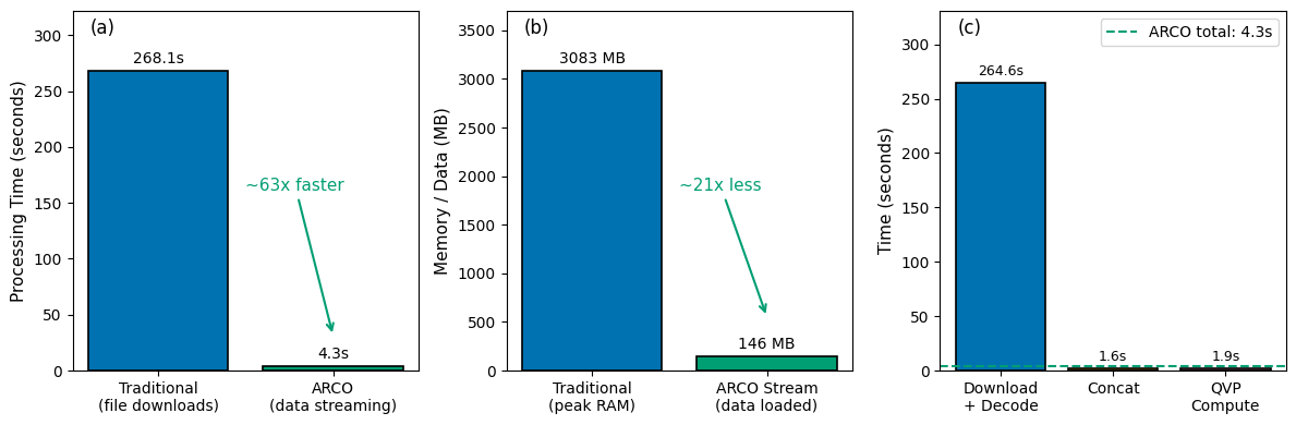
Now let’s compare the two approaches quantitatively. The figure below has three panels: (a) total processing time, (b) memory footprint (peak RAM vs ARCO bytes loaded), and © breakdown of the traditional workflow’s time among download/decode, concat, and QVP compute.

Show code cell source

Hide code cell source

t, a = metrics["traditional"], metrics["arco"]

# Throughput is measured against the *useful* bytes — the ones the QVP needs —
# so both paths are credited with delivering exactly the same product.
useful_mb = a["uncompressed_mb"]
t["throughput_mbs"] = useful_mb / t["total_workflow_time"]
a["throughput_mbs"] = useful_mb / a["total_time"]
metrics["speedup"] = t["total_workflow_time"] / a["total_time"]
metrics["data_reduction"] = t["uncompressed_mb"] / a["uncompressed_mb"]
metrics["throughput_gain"] = a["throughput_mbs"] / t["throughput_mbs"]

comparison = pd.DataFrame(
    [
        ("Total time [s]", f"{t['total_workflow_time']:.1f}", f"{a['total_time']:.1f}"),
        ("Timesteps", t["files_processed"], a["timesteps"]),
        (
            "Network transfer [MB]",
            f"{t['total_size_mb']:.0f} (gzip)",
            f"{useful_mb:.0f}",
        ),
        (
            "Decompressed / streamed [MB]",
            f"{t['uncompressed_mb']:.0f}",
            f"{useful_mb:.0f}",
        ),
        ("Peak RAM [MB]", f"{t['peak_memory_mb']:.0f}", f"{useful_mb:.0f}"),
        (
            "Throughput [MB/s]",
            f"{t['throughput_mbs']:.2f}",
            f"{a['throughput_mbs']:.1f}",
        ),
        ("Sweeps loaded", f"all ({N_TOTAL_SWEEPS}/file)", f"1 ({SELECTED_SWEEP})"),
        (
            "Variables loaded",
            f"all (~{N_TOTAL_VARS}/sweep)",
            f"{len(VARIABLES)} (selected)",
        ),
    ],
    columns=["Metric", "Traditional", "ARCO"],
).set_index("Metric")

print(
    f"{metrics['speedup']:.1f}× faster · "
    f"{metrics['data_reduction']:.0f}× less data loaded · "
    f"{metrics['throughput_gain']:.0f}× higher throughput"
)
comparison

25.0× faster · 22× less data loaded · 25× higher throughput

	Traditional	ARCO
Metric
Total time [s]	278.3	11.1
Timesteps	55	55
Network transfer [MB]	809 (gzip)	146
Decompressed / streamed [MB]	3236	146
Peak RAM [MB]	3083	146
Throughput [MB/s]	0.52	13.1
Sweeps loaded	all (17/file)	1 (sweep_16)
Variables loaded	all (~8/sweep)	4 (selected)

Show code cell source

Hide code cell source

BLUE, GREEN, ORANGE, PURPLE = "#0072B2", "#009E73", "#E69F00", "#CC79A7"  # Wong (2011)

plt.rcParams.update(
    {
        "font.family": "DejaVu Sans",
        "font.size": 10,
        "axes.titlesize": 12,
        "axes.labelsize": 11,
        "legend.fontsize": 10,
        "xtick.labelsize": 10,
        "ytick.labelsize": 10,
    }
)

fig, axes = plt.subplots(1, 3, figsize=(12, 4))
panels = [
    # labels, values, colours, ylabel, bar-label format, headroom, (note, arrow y-offset), fontsize
    (
        ["Traditional\n(file downloads)", "ARCO\n(data streaming)"],
        [t["total_workflow_time"], a["total_time"]],
        [BLUE, GREEN],
        "Processing Time (seconds)",
        "{:.1f}s",
        1.2,
        (f"~{metrics['speedup']:.0f}x faster", 35),
        10,
    ),
    (
        ["Traditional\n(peak RAM)", "ARCO Stream\n(data loaded)"],
        [t["peak_memory_mb"], a["uncompressed_mb"]],
        [BLUE, GREEN],
        "Memory / Data (MB)",
        "{:.0f} MB",
        1.2,
        (f"~{t['peak_memory_mb'] / a['uncompressed_mb']:.0f}x less", 500),
        10,
    ),
    (
        ["Download\n+ Decode", "Concat", "QVP\nCompute"],
        [t["total_time"], t["concat_time"], t["qvp_compute_time"]],
        [BLUE, ORANGE, PURPLE],
        "Time (seconds)",
        "{:.1f}s",
        1.25,
        None,
        9,
    ),
]

for ax, (labels, values, colors, ylabel, fmt, headroom, note, fontsize) in zip(
    axes, panels, strict=True
):
    bars = ax.bar(labels, values, color=colors, edgecolor="black", linewidth=1.2)
    ax.bar_label(
        bars, labels=[fmt.format(v) for v in values], padding=3, fontsize=fontsize
    )
    ax.set_ylabel(ylabel)
    ax.set_ylim(0, max(values) * headroom)
    if note:
        text, arrow_offset = note
        ax.annotate(
            text,
            # Offset keeps the arrowhead clear of the ARCO bar's own label.
            xy=(1, values[1] - max(values) * 0.03 + arrow_offset),
            xytext=(0.5, values[0] * 0.6),
            fontsize=11,
            color=GREEN,
            arrowprops=dict(arrowstyle="->", color=GREEN, lw=1.5),
        )

axes[2].axhline(
    a["total_time"],
    color=GREEN,
    linestyle="--",
    linewidth=1.5,
    label=f"ARCO total: {a['total_time']:.1f}s",
)
axes[2].legend(loc="upper right")
for ax, label in zip(axes, "abc", strict=True):
    ax.text(0.05, 0.98, f"({label})", transform=ax.transAxes, fontsize=12, va="top")

fig.tight_layout()
fig.savefig("workflow_comparison_cleaned.png", dpi=150, bbox_inches="tight")

---

Key takeaway

ARCO’s advantage isn’t compression — it’s selective access. The traditional path downloads every sweep of every variable in every file (~809 MB compressed, ~3.2 GB decompressed) to extract the 146 MB it actually needs. ARCO streams exactly those 146 MB and nothing else. Once the data model and storage layer make that selectivity declarative — one .sel(vcp_time=slice(...)) instead of fifty lines of file iteration — the toil Abernathey et al. (2021) describe simply disappears.

The same pattern scales linearly with window length. Notebook 4 picks up here and pushes it from a single 4-hour window to seasonal QPE on a Dask cluster.

---

← Notebook 2 — KLOT Low Sweeps   ·   Notebook 4 — QPE Scaling Benchmark →

References

• Abernathey, R.P., T. Augspurger, A. Banihirwe, C.C. Blackmon-Luca, T.J. Crone, C.L. Gentemann, J.J. Hamman, N. Henderson, C. Lepore, T.A. McCaie, N.H. Robinson, and R.P. Signell, 2021: Cloud-Native Repositories for Big Scientific Data. Computing in Science & Engineering, 23, 26–35, https://doi.org/10.1109/MCSE.2021.3059437.

• Ryzhkov, A., P. Zhang, H. Reeves, M. Kumjian, T. Tschallener, S. Trömel, and C. Simmer, 2016: Quasi-Vertical Profiles—A New Way to Look at Polarimetric Radar Data. J. Atmos. Oceanic Technol., 33, 551–562, https://doi.org/10.1175/JTECH-D-15-0020.1.

• Wilkinson, M.D., et al., 2016: The FAIR Guiding Principles for scientific data management and stewardship. Scientific Data, 3, 160018, https://doi.org/10.1038/sdata.2016.18.

• Ladino-Rincón, A., et al. (2026). Radar DataTree: A Cloud-Native AI-Ready Data Model for Accessible, Time-Aware Weather Radar Datasets. Submitted to IEEE Transactions on Big Data.

• Earlier preprint: arXiv:2510.24943, https://doi.org/10.48550/arXiv.2510.24943